
The cliche goes that the world is an increasingly interconnected place, and the connections between different entities are often best represented with a graph. Graphs are comprised of vertices (also often called “nodes”) and edges connecting those nodes. In this analysis, I’ll explore how to visualize networks using the igraph package in R.
I’ll visualize social networking data using anonymized data from Facebook; this data was originally curated in a recent paper about computing social circles in social networks. In our visualizations, the vertices in our network will represent Facebook users and the edges will represent these users being Facebook friends with each other.
The first file I’ll use, edges.csv, contains variables V1 and V2, which label the endpoints of edges in our network. Each row represents a pair of users in our graph who are Facebook friends. For a pair of friends A and B, edges.csv will only contain a single row – the smaller identifier will be listed first in this row. From this row, I’ll know that A is friends with B and B is friends with A.
The second file, users.csv, contains information about the Facebook users, who are the vertices in our network. This file contains the following variables:
- id: A unique identifier for this user; this is the value that appears in the rows of edges.csv
- gender: An identifier for the gender of a user taking the values A and B. Because the data is anonymized, we don’t know which value refers to males and which value refers to females.
- school: An identifier for the school the user attended taking the values A and AB (users with AB attended school A as well as another school B). Because the data is anonymized, we don’t know the schools represented by A and B.
- locale: An identifier for the locale of the user taking the values A and B. Because the data is anonymized, we don’t know which value refers to what locale.
Problem 1.1 - Summarizing the Data
Load the data from edges.csv into a dataframe called edges, and load the data from users.csv into a dataframe called users.
edges <- read.csv("edges.csv")
users <- read.csv("users.csv")
How many Facebook users are there in our dataset?
str(users)'data.frame': 59 obs. of 4 variables:
$ id : int 3981 3982 3983 3984 3985 3986 3987 3988 3989 3990 ...
$ gender: Factor w/ 3 levels "","A","B": 2 3 3 3 3 3 2 3 3 2 ...
$ school: Factor w/ 3 levels "","A","AB": 2 1 1 1 1 2 1 1 2 1 ...
$ locale: Factor w/ 3 levels "","A","B": 3 3 3 3 3 3 2 3 3 2 ...In our dataset, what is the average number of friends per user? Hint: this question is tricky, and it might help to start by thinking about a small example with two users who are friends.
head(edges) V1 V2
1 4019 4026
2 4023 4031
3 4023 4030
4 4027 4032
5 3988 4021
6 3982 3986edges[1,] # users 4019 and 4026 are friends V1 V2
1 4019 4026str(subset(edges, V1 == 4019)) # user 4019 has 2 connections as V1'data.frame': 2 obs. of 2 variables:
$ V1: int 4019 4019
$ V2: int 4026 4030str(subset(edges, V2 == 4019)) # user 4019 has 5 connections as V2'data.frame': 5 obs. of 2 variables:
$ V1: int 3997 3994 3998 4009 3981
$ V2: int 4019 4019 4019 4019 4019str(subset(edges, V1 == 4026)) # user 4026 has 1 connections as V1'data.frame': 1 obs. of 2 variables:
$ V1: int 4026
$ V2: int 4030str(subset(edges, V2 == 4026)) # user 4026 has 7 connections as V2'data.frame': 7 obs. of 2 variables:
$ V1: int 4019 4000 3995 4017 3986 3982 4021
$ V2: int 4026 4026 4026 4026 4026 4026 4026edges2 <- edges
edges2$PK <- row.names(edges2)
edges2 V1 V2 PK
1 4019 4026 1
2 4023 4031 2
3 4023 4030 3
4 4027 4032 4
5 3988 4021 5
6 3982 3986 6
7 3994 3998 7
8 3998 3999 8
9 3993 3995 9
10 3982 4021 10
11 3982 4037 11
12 3997 4019 12
13 3994 4019 13
14 3992 4017 14
15 3981 3998 15
16 3997 4018 16
17 4009 4030 17
18 3994 4018 18
19 3995 4000 19
20 4000 4026 20
21 4027 4038 21
22 4031 4038 22
23 4000 4021 23
24 3986 4030 24
25 3985 4014 25
26 3994 4030 26
27 3998 4021 27
28 3994 4009 28
29 3982 4023 29
30 3998 4019 30
31 4020 4031 31
32 4009 4023 32
33 3994 3997 33
34 3981 4023 34
35 3997 4030 35
36 3997 4021 36
37 4023 4034 37
38 3993 4004 38
39 3994 3996 39
40 4000 4030 40
41 3998 4014 41
42 4004 4013 42
43 4016 4025 43
44 3990 4016 44
45 3999 4005 45
46 4004 4023 46
47 4002 4020 47
48 3998 4018 48
49 3985 3995 49
50 3989 3991 50
51 4000 4017 51
52 4003 4009 52
53 3982 4030 53
54 3982 3994 54
55 3998 4005 55
56 3995 4014 56
57 4021 4030 57
58 594 4011 58
59 3993 4030 59
60 4020 4030 60
61 3989 4038 61
62 3989 4011 62
63 4009 4019 63
64 4004 4020 64
65 3995 4026 65
66 4017 4026 66
67 3989 4013 67
68 4020 4037 68
69 3998 4002 69
70 3995 4023 70
71 3983 4017 71
72 3999 4036 72
73 3982 3997 73
74 3990 4007 74
75 3985 3988 75
76 4018 4030 76
77 4026 4030 77
78 3997 4023 78
79 3996 4028 79
80 3982 3988 80
81 3988 4030 81
82 4013 4023 82
83 4014 4021 83
84 4014 4037 84
85 3986 4021 85
86 4017 4021 86
87 3982 4009 87
88 3998 4023 88
89 3998 4009 89
90 594 3989 90
91 3992 4000 91
92 4011 4031 92
93 4019 4030 93
94 4020 4038 94
95 3997 3998 95
96 4023 4038 96
97 4004 4031 97
98 4027 4031 98
99 4014 4038 99
100 3986 4000 100
101 3982 4003 101
102 3986 4033 102
103 3981 3994 103
104 4004 4038 104
105 3985 3993 105
106 4000 4033 106
107 4013 4038 107
108 4018 4023 108
109 4003 4030 109
110 3990 4025 110
111 3986 4026 111
112 3996 4002 112
113 4001 4029 113
114 4014 4030 114
115 4020 4027 115
116 3982 3998 116
117 3988 3993 117
118 4002 4031 118
119 3988 3995 119
120 3986 4014 120
121 4003 4023 121
122 3981 4019 122
123 3997 4009 123
124 4014 4023 124
125 4004 4030 125
126 4006 4027 126
127 594 4031 127
128 4007 4025 128
129 3981 4018 129
130 3981 3997 130
131 3982 4026 131
132 4014 4017 132
133 3991 4031 133
134 3987 4012 134
135 4007 4016 135
136 3995 4004 136
137 4017 4030 137
138 4002 4023 138
139 3994 4023 139
140 3982 4014 140
141 3981 4009 141
142 4021 4026 142
143 4013 4031 143
144 3986 4017 144
145 4002 4027 145
146 3985 4004 146Problem 1.2 - Summarizing the Data
Out of all the students who listed a school, what was the most common locale?
summary(users) id gender school locale
Min. : 594 : 2 :40 : 3
1st Qu.:3994 A:15 A :17 A: 6
Median :4009 B:42 AB: 2 B:50
Mean :3952
3rd Qu.:4024
Max. :4038 table(users$school, users$locale)
         A  B
      3  6 31
  A   0  0 17
  AB  0  0  2
Locale B
Problem 1.3 - Summarizing the Data
Is it possible that either school A or B is an all-girls or all-boys school?
table(users$gender, users$school)
        A AB
     1  1  0
  A 11  3  1
  B 28 13  1
No
Problem 2.1 - Creating a Network
We can create a new graph object using the graph.data.frame() function. Based on ?graph.data.frame, using the following code we will create a graph g describing our social network, with the attributes of each user correctly loaded.
?graph.data.frame
g <- graph.data.frame(edges, FALSE, users)
g
IGRAPH 097ec57 UN-- 59 146 --
+ attr: name (v/c), gender (v/c), school (v/c), locale (v/c)
+ edges from 097ec57 (vertex names):
[1] 4019--4026 4023--4031 4023--4030 4027--4032 3988--4021 3982--3986
[7] 3994--3998 3998--3999 3993--3995 3982--4021 3982--4037 3997--4019
[13] 3994--4019 3992--4017 3981--3998 3997--4018 4009--4030 3994--4018
[19] 3995--4000 4000--4026 4027--4038 4031--4038 4000--4021 3986--4030
[25] 3985--4014 3994--4030 3998--4021 3994--4009 3982--4023 3998--4019
[31] 4020--4031 4009--4023 3994--3997 3981--4023 3997--4030 3997--4021
[37] 4023--4034 3993--4004 3994--3996 4000--4030 3998--4014 4004--4013
[43] 4016--4025 3990--4016 3999--4005 4004--4023 4002--4020 3998--4018
+ ... omitted several edgesNote: A directed graph is one where the edges only go one way – they point from one vertex to another. The other option is an undirected graph, which means that the relations between the vertices are symmetric.
Now, we want to plot our graph. By default, the vertices are large and have text labels of a user’s identifier, this would clutter the output.
We will plot with no text labels and smaller vertices:
plot(g, vertex.size=5, vertex.label=NA)
In this graph, there are a number of groups of nodes where all the nodes in each group are connected but, the groups are disjoint from one another, forming “islands” in the graph. Such groups are called “connected components,” or “components” for short.
How many connected components with at least 2 nodes are there in the graph? #### 4
How many users are there with no friends in the network? #### 7
Problem 2.3 - Creating a Network
In our graph, the “degree” of a node is its number of friends. We have already seen that some nodes in our graph have degree 0 (these are the nodes with no friends), while others have much higher degree. We can use degree(g) to compute the degree of all the nodes in our graph g.
degree(g)3981 3982 3983 3984 3985 3986 3987 3988 3989 3990 3991 3992 3993 3994 3995
7 13 1 0 5 8 1 6 5 3 2 2 5 10 8
594 3996 3997 3998 3999 4000 4001 4002 4003 4004 4005 4006 4007 4008 4009
3 3 10 13 3 8 1 6 4 9 2 1 3 0 9
4010 4011 4012 4013 4014 4015 4016 4017 4018 4019 4020 4021 4022 4023 4024
0 3 1 5 11 0 3 8 6 7 7 10 0 17 0
4025 4026 4027 4028 4029 4030 4031 4032 4033 4034 4035 4036 4037 4038
3 8 6 1 1 18 10 1 2 1 0 1 3 8 How many users are friends with 10 or more other Facebook users in this network?
sum(degree(g) >= 10)[1] 9Problem 2.4 - Creating a Network
In a network, it’s often visually useful to draw attention to “important” nodes in the network. While this might mean different things in different contexts, in a social network we might consider a user with a large number of friends to be an important user. From the previous problem, we know this is the same as saying that nodes with a high degree are important users.
To visually draw attention to these nodes, we will change the size of the vertices so the vertices with high degrees are larger. To do this, we will change the “size” attribute of the vertices of our graph to be an increasing function of their degrees:
V(g)$size <- degree(g)/2+2Now, that we have specified the vertex size of each vertex, we will no longer use the vertex.size parameter when we plot our graph:
plot(g, vertex.label=NA)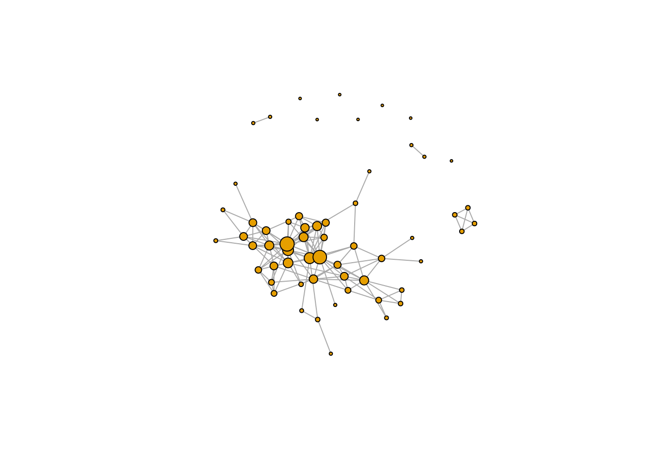
What is the largest size we assigned to any node in our graph?
max(V(g)$size)[1] 11What is the smallest size we assigned to any node in our graph?
min(V(g)$size)[1] 2Problem 3.1 - Coloring Vertices
Thus far, we have changed the “size” attributes of our vertices. However, we can also change the colors of vertices to capture additional information about the Facebook users we are depicting.
When changing the size of nodes, we first obtained the vertices of our graph with V(g) and then accessed the the size attribute with V(g)\(size. To change the color, we will update the attribute V(g)\)color.
To color the vertices based on the gender of the user, we will need access to that variable. When we created our graph g, we provided it with the dataframe users, which had variables gender, school, and locale. These are now stored as attributes V(g)\(gender, V(g)\)school, and V(g)$locale.
We can update the colors by setting the color to black for all vertices, than setting it to red for the vertices with gender A and setting it to gray for the vertices with gender B:
V(g)$color = "black"
V(g)$color[V(g)$gender == "A"] = "red"
V(g)$color[V(g)$gender == "B"] = "gray"
Ploting the resulting graph.
What is the gender of the users with the highest degree in the graph?
plot(g, vertex.label=NA)
Gender B
Problem 3.2 - Coloring Vertices
Now, color the vertices based on the school that each user in our network attended.
table(V(g)$school)
    A AB
40 17  2
V(g)$color = "black"
V(g)$color[V(g)$school == "A"] = "red"
V(g)$color[V(g)$school == "AB"] = "gray"
plot(g, vertex.label=NA)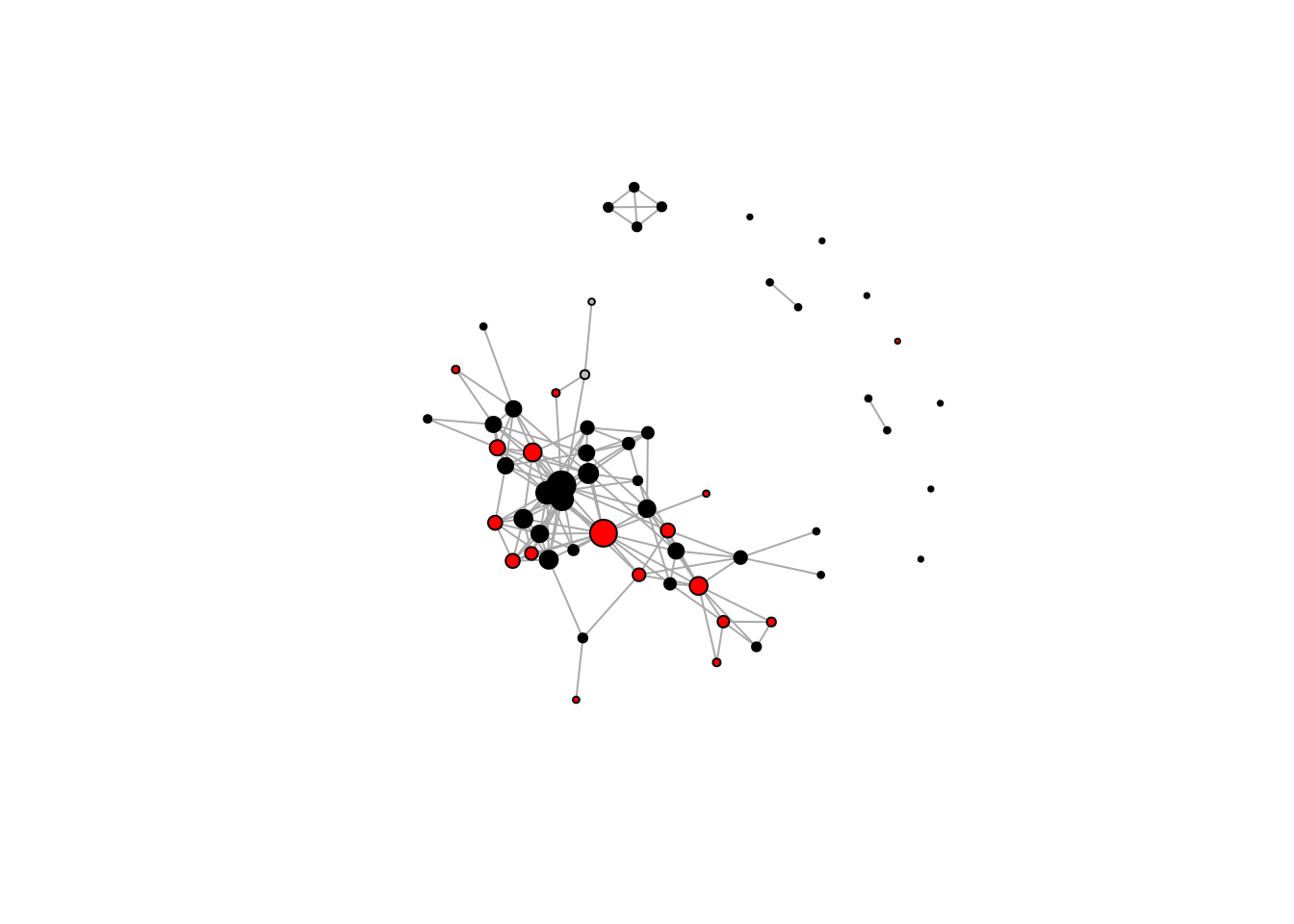
Are the two users who attended both schools A and B Facebook friends with each other? #### Yes
What best describes the users with highest degree? #### Some, but not all, of the high-degree users attended school A
Problem 3.3 - Coloring Vertices
Now, color the vertices based on the locale of the user.
table(V(g)$locale)
    A  B
 3  6 50
V(g)$color = "black"
V(g)$color[V(g)$locale == "A"] = "red"
V(g)$color[V(g)$locale == "B"] = "gray"
plot(g, vertex.label=NA)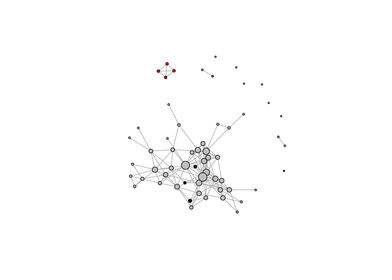
The large connected component is most associated with which locale? #### Locale B
The 4-user connected component is most associated with which locale? #### Locale A
Problem 4 - Other Plotting Options
The help page is a helpful tool when making visualizations. The following questions with the help of ?igraph.plotting and experimentation in our R console.
?igraph.plottingWhich igraph plotting function would enable us to plot our graph in 3-D?
?rglplotrglplot
What parameter to the plot() function would we use to change the edge width when plotting g?
?plot.igraphedge.width
)