Letter Reecognition

Apr 8, 2019

One of the earliest applications of predictive analytics methods applied so far was to automatically recognize letters, which post office machines use to sort mail. In this analysis, I’ll build a model that uses statistics of images of four letters in the Roman alphabet – A, B, P, and R – to predict which letter a particular image corresponds to.

Note, that this is a multiclass classification problem. We have mostly focused on binary classification problems (e.g., predicting whether an individual voted or not, whether the Supreme Court will affirm or reverse a case, whether or not a person is at risk for a certain disease, etc.). In this problem, we have more than two classifications that are possible for each observation.

The file letters_ABPR.csv contains 3116 observations, each of which corresponds to a certain image of one of the four letters A, B, P and R. The images came from 20 different fonts, which were then randomly distorted to produce the final images; each such distorted image is represented as a collection of pixels, each of which is “on” or “off”.

For each such distorted image, we have available certain statistics of the image in terms of these pixels, as well as which of the four letters the image is. This data comes from the UCI ML Repository.

This dataset contains the following 17 variables:

letter = the letter that the image corresponds to (A, B, P or R)
xbox = the horizontal position of where the smallest box covering the letter shape begins.
ybox = the vertical position of where the smallest box covering the letter shape begins.
width = the width of this smallest box.
height = the height of this smallest box.
onpix = the total number of “on” pixels in the character image
xbar = the mean horizontal position of all of the “on” pixels
ybar = the mean vertical position of all of the “on” pixels
x2bar = the mean squared horizontal position of all of the “on” pixels in the image
y2bar = the mean squared vertical position of all of the “on” pixels in the image
xybar = the mean of the product of the horizontal and vertical position of all of the “on” pixels in the image
x2ybar = the mean of the product of the squared horizontal position and the vertical position of all of the “on” pixels
xy2bar = the mean of the product of the horizontal position and the squared vertical position of all of the “on” pixels
xedge = the mean number of edges (the number of times an “off” pixel is followed by an “on” pixel, or the image boundary is hit) as the image is scanned from left to right, along the whole vertical length of the image
xedgeycor = the mean of the product of the number of horizontal edges at each vertical position and the vertical position
yedge = the mean number of edges as the images is scanned from top to bottom, along the whole horizontal length of the image
yedgexcor = the mean of the product of the number of vertical edges at each horizontal position and the horizontal position

Load the dataset

letters <- read.csv("letters_ABPR.csv")
summary(letters)

 letter       xbox             ybox            width       
 A:789   Min.   : 0.000   Min.   : 0.000   Min.   : 1.000  
 B:766   1st Qu.: 3.000   1st Qu.: 5.000   1st Qu.: 4.000  
 P:803   Median : 4.000   Median : 7.000   Median : 5.000  
 R:758   Mean   : 3.915   Mean   : 7.051   Mean   : 5.186  
         3rd Qu.: 5.000   3rd Qu.: 9.000   3rd Qu.: 6.000  
         Max.   :13.000   Max.   :15.000   Max.   :11.000  
     height           onpix             xbar             ybar       
 Min.   : 0.000   Min.   : 0.000   Min.   : 3.000   Min.   : 0.000  
 1st Qu.: 4.000   1st Qu.: 2.000   1st Qu.: 6.000   1st Qu.: 6.000  
 Median : 6.000   Median : 4.000   Median : 7.000   Median : 7.000  
 Mean   : 5.276   Mean   : 3.869   Mean   : 7.469   Mean   : 7.197  
 3rd Qu.: 7.000   3rd Qu.: 5.000   3rd Qu.: 8.000   3rd Qu.: 9.000  
 Max.   :12.000   Max.   :12.000   Max.   :14.000   Max.   :15.000  
     x2bar            y2bar           xybar            x2ybar     
 Min.   : 0.000   Min.   :0.000   Min.   : 3.000   Min.   : 0.00  
 1st Qu.: 3.000   1st Qu.:2.000   1st Qu.: 7.000   1st Qu.: 3.00  
 Median : 4.000   Median :4.000   Median : 8.000   Median : 5.00  
 Mean   : 4.706   Mean   :3.903   Mean   : 8.491   Mean   : 4.52  
 3rd Qu.: 6.000   3rd Qu.:5.000   3rd Qu.:10.000   3rd Qu.: 6.00  
 Max.   :11.000   Max.   :8.000   Max.   :14.000   Max.   :10.00  
     xy2bar           xedge          xedgeycor          yedge     
 Min.   : 0.000   Min.   : 0.000   Min.   : 1.000   Min.   : 0.0  
 1st Qu.: 6.000   1st Qu.: 2.000   1st Qu.: 7.000   1st Qu.: 3.0  
 Median : 7.000   Median : 2.000   Median : 8.000   Median : 4.0  
 Mean   : 6.711   Mean   : 2.913   Mean   : 7.763   Mean   : 4.6  
 3rd Qu.: 8.000   3rd Qu.: 4.000   3rd Qu.: 9.000   3rd Qu.: 6.0  
 Max.   :14.000   Max.   :10.000   Max.   :13.000   Max.   :12.0  
   yedgexcor     
 Min.   : 1.000  
 1st Qu.: 7.000  
 Median : 8.000  
 Mean   : 8.418  
 3rd Qu.:10.000  
 Max.   :13.000

str(letters)

'data.frame':   3116 obs. of  17 variables:
 $ letter   : Factor w/ 4 levels "A","B","P","R": 2 1 4 2 3 4 4 1 3 3 ...
 $ xbox     : int  4 1 5 5 3 8 2 3 8 6 ...
 $ ybox     : int  2 1 9 9 6 10 6 7 14 10 ...
 $ width    : int  5 3 5 7 4 8 4 5 7 8 ...
 $ height   : int  4 2 7 7 4 6 4 5 8 8 ...
 $ onpix    : int  4 1 6 10 2 6 3 3 4 7 ...
 $ xbar     : int  8 8 6 9 4 7 6 12 5 8 ...
 $ ybar     : int  7 2 11 8 14 7 7 2 10 5 ...
 $ x2bar    : int  6 2 7 4 8 3 5 3 6 7 ...
 $ y2bar    : int  6 2 3 4 1 5 5 2 3 5 ...
 $ xybar    : int  7 8 7 6 11 8 6 10 12 7 ...
 $ x2ybar   : int  6 2 3 8 6 4 5 2 5 6 ...
 $ xy2bar   : int  6 8 9 6 3 8 7 9 4 6 ...
 $ xedge    : int  2 1 2 6 0 6 3 2 4 3 ...
 $ xedgeycor: int  8 6 7 11 10 6 7 6 10 9 ...
 $ yedge    : int  7 2 5 8 4 7 5 3 4 8 ...
 $ yedgexcor: int  10 7 11 7 8 7 8 8 8 9 ...

Problem 1.1 - Predicting B or not B

Let’s warm up by attempting to predict just whether a letter is B or not. To begin, load the file letters_ABPR.csv into R, and call it letters. Then, create a new variable isB in the dataframe, which takes the value “TRUE” if the observation corresponds to the letter B, and “FALSE” if it does not.

letters$isB <- as.factor(letters$letter == "B")

Now, split the dataset into a training and testing set, putting 50% of the data in the training set. Set the seed to 1000 before making the split. The first argument to sample.split should be the dependent variable “letters$isB”. Remember that TRUE values from sample.split should go in the training set.

library(caTools)
set.seed(1000)
lettersSplit = sample.split(letters$isB, SplitRatio = 0.5)
lettersTrain = subset(letters, lettersSplit == TRUE)
lettersTest = subset(letters, lettersSplit == FALSE)

Before building models, let’s consider a baseline method that always predicts the most frequent outcome, which is “not B”.

What is the accuracy of this baseline method on the test set?

table(letters$isB)


FALSE  TRUE 
 2350   766

table(lettersTest$isB)


FALSE  TRUE 
 1175   383

1175 / (1175 + 383)

[1] 0.754172

Problem 1.2 - Predicting B or not B

Now, build a classification tree to predict whether a letter is a B or not, using the training set to build the model. Remember to remove the variable “letter” out of the model, as this is related to what we are trying to predict!

library(rpart)
library(rpart.plot)
CARTb <- rpart(isB ~ . - letter, data = lettersTrain, method="class")

We are just using the default parameters in our CART model, so we don’t need to add the minbucket or cp arguments at all. We also added the argument method=“class” since this is a classification problem.

What is the accuracy of the CART model on the test-set? (Use type=“class” when making predictions on the test set.)

bPredict <- predict(CARTb, newdata = lettersTest, type = "class")
table(lettersTest$isB, bPredict)

       bPredict
        FALSE TRUE
  FALSE  1118   57
  TRUE     43  340

(1126 + 342) / nrow(lettersTest)

[1] 0.9422336

Problem 1.3 - Predicting B or Not B

Now, build a random forest model to predict whether the letter is a B or not (the isB variable) using the training set. Using all of the other variables as independent variables, except letter (since it helped us define what we are trying to predict!). Using the default settings for ntree and nodesize (don’t include these arguments at all). Right before building the model, set the seed to 1000. (NOTE: You might get a slightly different answer on this problem, even if you set the random seed. This has to do with your operating system and the implementation of the random forest algorithm.)

What is the accuracy of the model on the test set?

bForestPredict <- predict(bForest, newdata = lettersTest, type = "class")
table(lettersTest$isB, bForestPredict)

       bForestPredict
        FALSE TRUE
  FALSE  1163   12
  TRUE      9  374

(1164 + 372) / nrow(lettersTest)

[1] 0.9858793

Random forests tends to improve on CART in terms of predictive accuracy. Sometimes, this improvement can be quite significant, as it is here.

Problem 2.1 - Predicting the letters A, B, P, R

Let us now move on to the problem that we were originally interested in, which is to predict whether or not a letter is one of the four letters A, B, P or R.

As we saw earlier, building a multiclass classification CART model is no harder than building the models for binary classification problems. Fortunately, building a random forest model is just as easy. The variable in our dataframe which we will be trying to predict is “letter”.

Start by converting letter in the original dataset (letters) to a factor by running the following code:

letters$letter <- as.factor(letters$letter)

Now, generate new training and testing sets of the letters dataframe using letters$letter as the first input to the sample.split function. Before splitting, set your seed to 2000. Again put 50% of the data in the training set. (Why do we need to split the data again? Remember that sample.split balances the outcome variable in the training and testing sets. With a new outcome variable, we want to re-generate our split.)

set.seed(2000)
lettersAllSplit <- sample.split(letters$letter, SplitRatio = 0.5)
lettersAllTrain <- subset(letters, lettersAllSplit == TRUE)
lettersAllTest <- subset(letters, lettersAllSplit == FALSE)

In a multiclass classification problem, a simple baseline model is to predict the most frequent class of all of the options.

What is the baseline accuracy on the testing set?

table(letters$letter)


  A   B   P   R 
789 766 803 758

table(lettersAllTest$letter)


  A   B   P   R 
395 383 401 379

401 / nrow(lettersAllTest)

[1] 0.2573813

P is the most frequent class in the test set

Problem 2.2 - Predicting the letters A, B, P, R

Now build a classification tree to predict “letter”, using the training set to build our model. You should use all of the other variables as independent variables, except “isB”, since it is related to what we are trying to predict!

Just use the default parameters in your CART model. Add the argument method=“class” since this is a classification problem. Even though we have multiple classes here, nothing changes in how we build the model from the binary case.

CARTletters <- rpart(letter ~ . - isB, data = lettersAllTrain, method="class")
summary(CARTletters)

Call:
rpart(formula = letter ~ . - isB, data = lettersAllTrain, method = "class")
  n= 1558 

          CP nsplit rel error    xerror       xstd
1 0.31920415      0 1.0000000 1.0346021 0.01442043
2 0.25865052      1 0.6807958 0.6323529 0.01704001
3 0.18685121      2 0.4221453 0.4238754 0.01585412
4 0.02595156      3 0.2352941 0.2370242 0.01299919
5 0.02076125      4 0.2093426 0.2162630 0.01253234
6 0.01730104      5 0.1885813 0.1980969 0.01209034
7 0.01384083      6 0.1712803 0.1894464 0.01186782
8 0.01211073      7 0.1574394 0.1678201 0.01127370
9 0.01000000      8 0.1453287 0.1608997 0.01107113

Variable importance
     ybar xedgeycor    x2ybar    xy2bar     yedge     y2bar     xedge 
       17        16        14        12        11         8         7 
    xybar     x2bar      xbar 
        5         5         3 

Node number 1: 1558 observations,    complexity param=0.3192042
  predicted class=P  expected loss=0.7419769  P(node) =1
    class counts:   394   383   402   379
   probabilities: 0.253 0.246 0.258 0.243 
  left son=2 (1088 obs) right son=3 (470 obs)
  Primary splits:
      xedgeycor < 8.5  to the left,  improve=293.2010, (0 missing)
      ybar      < 5.5  to the left,  improve=287.8322, (0 missing)
      xy2bar    < 5.5  to the right, improve=278.1742, (0 missing)
      x2ybar    < 2.5  to the left,  improve=262.6356, (0 missing)
      yedge     < 4.5  to the left,  improve=177.0582, (0 missing)
  Surrogate splits:
      xy2bar < 5.5  to the right, agree=0.892, adj=0.643, (0 split)
      ybar   < 8.5  to the left,  agree=0.821, adj=0.406, (0 split)
      xedge  < 1.5  to the right, agree=0.816, adj=0.391, (0 split)
      xybar  < 10.5 to the left,  agree=0.785, adj=0.287, (0 split)
      x2ybar < 6.5  to the left,  agree=0.777, adj=0.262, (0 split)

Node number 2: 1088 observations,    complexity param=0.2586505
  predicted class=A  expected loss=0.6488971  P(node) =0.6983312
    class counts:   382   338    13   355
   probabilities: 0.351 0.311 0.012 0.326 
  left son=4 (344 obs) right son=5 (744 obs)
  Primary splits:
      ybar      < 5.5  to the left,  improve=275.7625, (0 missing)
      x2ybar    < 2.5  to the left,  improve=240.6702, (0 missing)
      y2bar     < 2.5  to the left,  improve=226.4519, (0 missing)
      yedge     < 3.5  to the left,  improve=215.2610, (0 missing)
      xedgeycor < 7.5  to the right, improve=171.4917, (0 missing)
  Surrogate splits:
      x2ybar < 2.5  to the left,  agree=0.904, adj=0.698, (0 split)
      y2bar  < 2.5  to the left,  agree=0.892, adj=0.657, (0 split)
      yedge  < 3.5  to the left,  agree=0.881, adj=0.625, (0 split)
      x2bar  < 2.5  to the left,  agree=0.820, adj=0.430, (0 split)
      xbar   < 9.5  to the right, agree=0.779, adj=0.302, (0 split)

Node number 3: 470 observations,    complexity param=0.01730104
  predicted class=P  expected loss=0.1723404  P(node) =0.3016688
    class counts:    12    45   389    24
   probabilities: 0.026 0.096 0.828 0.051 
  left son=6 (91 obs) right son=7 (379 obs)
  Primary splits:
      xybar  < 7.5  to the left,  improve=59.48719, (0 missing)
      xy2bar < 6.5  to the right, improve=54.86112, (0 missing)
      ybar   < 7.5  to the left,  improve=49.49367, (0 missing)
      yedge  < 6.5  to the right, improve=48.42295, (0 missing)
      xedge  < 5.5  to the left,  improve=30.83057, (0 missing)
  Surrogate splits:
      xy2bar < 6.5  to the right, agree=0.936, adj=0.670, (0 split)
      ybar   < 7.5  to the left,  agree=0.902, adj=0.495, (0 split)
      xedge  < 5.5  to the right, agree=0.889, adj=0.429, (0 split)
      yedge  < 6.5  to the right, agree=0.885, adj=0.407, (0 split)
      onpix  < 6.5  to the right, agree=0.838, adj=0.165, (0 split)

Node number 4: 344 observations
  predicted class=A  expected loss=0.04360465  P(node) =0.2207959
    class counts:   329     9     3     3
   probabilities: 0.956 0.026 0.009 0.009 

Node number 5: 744 observations,    complexity param=0.1868512
  predicted class=R  expected loss=0.5268817  P(node) =0.4775353
    class counts:    53   329    10   352
   probabilities: 0.071 0.442 0.013 0.473 
  left son=10 (342 obs) right son=11 (402 obs)
  Primary splits:
      xedgeycor < 7.5  to the right, improve=139.70670, (0 missing)
      xy2bar    < 7.5  to the left,  improve= 92.43059, (0 missing)
      x2ybar    < 5.5  to the right, improve= 81.07422, (0 missing)
      y2bar     < 4.5  to the right, improve= 56.45671, (0 missing)
      yedgexcor < 10.5 to the left,  improve= 52.58754, (0 missing)
  Surrogate splits:
      x2ybar < 5.5  to the right, agree=0.738, adj=0.430, (0 split)
      xy2bar < 6.5  to the left,  agree=0.675, adj=0.292, (0 split)
      xedge  < 2.5  to the left,  agree=0.675, adj=0.292, (0 split)
      yedge  < 5.5  to the right, agree=0.644, adj=0.225, (0 split)
      ybar   < 7.5  to the left,  agree=0.625, adj=0.184, (0 split)

Node number 6: 91 observations,    complexity param=0.01384083
  predicted class=B  expected loss=0.5604396  P(node) =0.05840822
    class counts:    10    40    20    21
   probabilities: 0.110 0.440 0.220 0.231 
  left son=12 (55 obs) right son=13 (36 obs)
  Primary splits:
      x2bar     < 3.5  to the right, improve=14.308240, (0 missing)
      xy2bar    < 7.5  to the left,  improve= 9.472092, (0 missing)
      yedge     < 4.5  to the left,  improve= 9.449763, (0 missing)
      x2ybar    < 7.5  to the right, improve= 8.053076, (0 missing)
      yedgexcor < 6.5  to the right, improve= 7.478284, (0 missing)
  Surrogate splits:
      yedgexcor < 5.5  to the right, agree=0.736, adj=0.333, (0 split)
      x2ybar    < 7.5  to the left,  agree=0.725, adj=0.306, (0 split)
      yedge     < 5.5  to the right, agree=0.725, adj=0.306, (0 split)
      xy2bar    < 8.5  to the left,  agree=0.714, adj=0.278, (0 split)
      ybar      < 7.5  to the left,  agree=0.681, adj=0.194, (0 split)

Node number 7: 379 observations
  predicted class=P  expected loss=0.02638522  P(node) =0.2432606
    class counts:     2     5   369     3
   probabilities: 0.005 0.013 0.974 0.008 

Node number 10: 342 observations,    complexity param=0.02595156
  predicted class=B  expected loss=0.2192982  P(node) =0.2195122
    class counts:    14   267    10    51
   probabilities: 0.041 0.781 0.029 0.149 
  left son=20 (283 obs) right son=21 (59 obs)
  Primary splits:
      xy2bar    < 7.5  to the left,  improve=48.65030, (0 missing)
      xedge     < 2.5  to the left,  improve=33.98799, (0 missing)
      y2bar     < 4.5  to the right, improve=27.13499, (0 missing)
      yedgexcor < 6.5  to the left,  improve=15.49245, (0 missing)
      ybar      < 8.5  to the left,  improve=15.03303, (0 missing)
  Surrogate splits:
      xedge     < 5.5  to the left,  agree=0.871, adj=0.254, (0 split)
      yedgexcor < 4.5  to the right, agree=0.854, adj=0.153, (0 split)
      ybar      < 9.5  to the left,  agree=0.848, adj=0.119, (0 split)
      xbox      < 6.5  to the left,  agree=0.842, adj=0.085, (0 split)
      ybox      < 11.5 to the left,  agree=0.842, adj=0.085, (0 split)

Node number 11: 402 observations,    complexity param=0.02076125
  predicted class=R  expected loss=0.2512438  P(node) =0.2580231
    class counts:    39    62     0   301
   probabilities: 0.097 0.154 0.000 0.749 
  left son=22 (26 obs) right son=23 (376 obs)
  Primary splits:
      yedge     < 2.5  to the left,  improve=35.46191, (0 missing)
      x2ybar    < 0.5  to the left,  improve=34.14932, (0 missing)
      y2bar     < 1.5  to the left,  improve=33.87850, (0 missing)
      x2bar     < 3.5  to the left,  improve=19.57685, (0 missing)
      yedgexcor < 8.5  to the left,  improve=19.07812, (0 missing)
  Surrogate splits:
      y2bar  < 1.5  to the left,  agree=0.993, adj=0.885, (0 split)
      x2ybar < 0.5  to the left,  agree=0.993, adj=0.885, (0 split)

Node number 12: 55 observations
  predicted class=B  expected loss=0.3090909  P(node) =0.03530167
    class counts:     1    38    13     3
   probabilities: 0.018 0.691 0.236 0.055 

Node number 13: 36 observations
  predicted class=R  expected loss=0.5  P(node) =0.02310655
    class counts:     9     2     7    18
   probabilities: 0.250 0.056 0.194 0.500 

Node number 20: 283 observations
  predicted class=B  expected loss=0.08480565  P(node) =0.1816431
    class counts:     3   259     8    13
   probabilities: 0.011 0.915 0.028 0.046 

Node number 21: 59 observations
  predicted class=R  expected loss=0.3559322  P(node) =0.03786906
    class counts:    11     8     2    38
   probabilities: 0.186 0.136 0.034 0.644 

Node number 22: 26 observations
  predicted class=A  expected loss=0.03846154  P(node) =0.01668806
    class counts:    25     0     0     1
   probabilities: 0.962 0.000 0.000 0.038 

Node number 23: 376 observations,    complexity param=0.01211073
  predicted class=R  expected loss=0.2021277  P(node) =0.241335
    class counts:    14    62     0   300
   probabilities: 0.037 0.165 0.000 0.798 
  left son=46 (26 obs) right son=47 (350 obs)
  Primary splits:
      yedge  < 7.5  to the right, improve=19.73450, (0 missing)
      x2ybar < 5.5  to the right, improve=16.32647, (0 missing)
      xybar  < 8.5  to the right, improve=15.20779, (0 missing)
      xedge  < 3.5  to the right, improve=14.35240, (0 missing)
      onpix  < 4.5  to the right, improve=12.94437, (0 missing)
  Surrogate splits:
      xedgeycor < 4.5  to the left,  agree=0.939, adj=0.115, (0 split)

Node number 46: 26 observations
  predicted class=B  expected loss=0.3076923  P(node) =0.01668806
    class counts:     4    18     0     4
   probabilities: 0.154 0.692 0.000 0.154 

Node number 47: 350 observations
  predicted class=R  expected loss=0.1542857  P(node) =0.224647
    class counts:    10    44     0   296
   probabilities: 0.029 0.126 0.000 0.846

prp(CARTletters)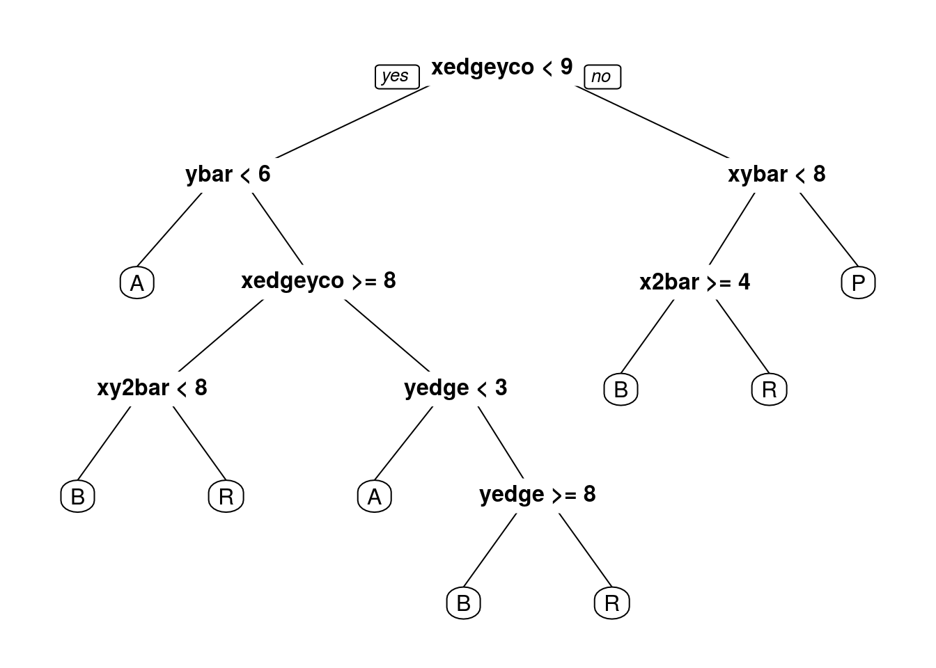

What is the test-set accuracy of our CART model? Use the argument type=“class” when making predictions. (HINT: When you are computing the test-set accuracy using the confusion matrix, you want to add everything on the main diagonal and divide by the total number of observations in the test-set, which can be computed with nrow(test), where test is the name of our test-set).

lettersPredict <- 
    as.vector(predict(CARTletters, newdata = lettersAllTest, type = "class"))
length(lettersPredict)

[1] 1558

lettersPredict

   [1] "B" "R" "A" "P" "A" "R" "A" "A" "A" "B" "A" "A" "P" "P" "B" "R" "B"
  [18] "P" "P" "B" "A" "A" "B" "P" "R" "R" "A" "A" "B" "P" "A" "B" "P" "B"
  [35] "B" "A" "P" "B" "B" "R" "A" "R" "R" "R" "R" "B" "B" "B" "P" "R" "P"
  [52] "B" "R" "R" "B" "B" "R" "A" "R" "P" "R" "P" "B" "R" "B" "A" "P" "P"
  [69] "R" "R" "A" "B" "P" "R" "R" "R" "A" "P" "R" "R" "P" "B" "B" "R" "A"
  [86] "P" "A" "A" "A" "P" "A" "A" "A" "B" "B" "B" "R" "R" "P" "P" "B" "A"
 [103] "R" "P" "R" "R" "B" "A" "P" "P" "R" "P" "A" "A" "P" "R" "P" "R" "P"
 [120] "B" "R" "R" "R" "B" "R" "A" "P" "A" "B" "P" "P" "P" "B" "R" "A" "P"
 [137] "P" "R" "B" "R" "R" "A" "B" "A" "P" "R" "R" "A" "R" "A" "B" "B" "B"
 [154] "B" "B" "P" "A" "P" "R" "R" "A" "A" "P" "A" "A" "P" "B" "B" "B" "P"
 [171] "P" "B" "R" "B" "R" "P" "B" "P" "B" "A" "P" "A" "A" "B" "R" "P" "P"
 [188] "P" "R" "A" "B" "B" "A" "R" "B" "R" "P" "R" "A" "R" "A" "A" "R" "R"
 [205] "B" "R" "B" "A" "B" "P" "R" "A" "A" "R" "B" "R" "A" "R" "P" "R" "R"
 [222] "B" "P" "P" "A" "A" "B" "P" "B" "P" "R" "P" "A" "R" "R" "R" "A" "A"
 [239] "B" "P" "R" "R" "A" "R" "A" "P" "B" "R" "P" "B" "A" "R" "B" "A" "A"
 [256] "A" "B" "B" "A" "P" "A" "B" "P" "R" "A" "R" "P" "B" "P" "R" "P" "A"
 [273] "R" "R" "R" "B" "R" "R" "P" "R" "P" "P" "A" "R" "P" "R" "R" "A" "P"
 [290] "B" "A" "A" "A" "A" "B" "R" "R" "A" "P" "R" "B" "P" "A" "R" "R" "R"
 [307] "R" "A" "B" "B" "R" "P" "R" "B" "A" "A" "P" "R" "A" "B" "P" "A" "R"
 [324] "B" "R" "P" "P" "A" "P" "R" "A" "R" "A" "B" "P" "R" "P" "R" "P" "B"
 [341] "B" "B" "A" "A" "B" "B" "B" "P" "P" "P" "B" "B" "A" "P" "R" "R" "R"
 [358] "R" "P" "B" "P" "B" "P" "R" "B" "P" "B" "R" "B" "A" "P" "R" "R" "P"
 [375] "B" "B" "R" "A" "R" "A" "R" "R" "A" "B" "P" "R" "A" "P" "P" "A" "A"
 [392] "A" "P" "R" "R" "P" "B" "A" "A" "R" "P" "A" "R" "B" "A" "P" "P" "P"
 [409] "B" "A" "R" "P" "R" "P" "A" "A" "R" "P" "P" "R" "R" "R" "B" "R" "P"
 [426] "B" "A" "R" "R" "P" "P" "A" "A" "B" "A" "P" "P" "B" "P" "A" "R" "B"
 [443] "P" "B" "R" "P" "A" "A" "B" "P" "B" "R" "A" "P" "A" "R" "P" "P" "P"
 [460] "R" "B" "B" "P" "P" "R" "B" "R" "B" "P" "R" "B" "A" "R" "B" "P" "B"
 [477] "R" "R" "P" "R" "B" "B" "A" "P" "B" "P" "P" "B" "A" "A" "A" "B" "P"
 [494] "P" "R" "B" "A" "A" "B" "A" "R" "R" "R" "B" "R" "B" "B" "R" "R" "A"
 [511] "A" "P" "R" "P" "A" "R" "B" "A" "P" "P" "R" "P" "B" "B" "A" "A" "P"
 [528] "A" "B" "P" "A" "P" "A" "R" "A" "A" "R" "R" "P" "R" "A" "R" "R" "R"
 [545] "B" "B" "R" "R" "R" "R" "A" "B" "R" "P" "B" "A" "A" "R" "R" "R" "R"
 [562] "R" "R" "P" "A" "P" "R" "A" "R" "R" "R" "B" "R" "B" "B" "A" "R" "P"
 [579] "B" "R" "B" "R" "P" "B" "A" "A" "B" "R" "A" "A" "B" "P" "P" "B" "B"
 [596] "B" "P" "R" "A" "P" "P" "B" "B" "P" "B" "R" "P" "P" "P" "R" "A" "A"
 [613] "B" "P" "B" "B" "R" "B" "A" "B" "A" "P" "R" "R" "A" "P" "B" "A" "P"
 [630] "A" "P" "R" "R" "P" "B" "R" "A" "A" "A" "B" "B" "P" "B" "A" "P" "P"
 [647] "P" "B" "A" "P" "P" "R" "P" "P" "R" "R" "B" "R" "A" "P" "B" "P" "P"
 [664] "A" "P" "A" "R" "P" "P" "R" "A" "R" "P" "A" "B" "B" "R" "P" "P" "R"
 [681] "A" "P" "B" "P" "R" "P" "A" "A" "A" "R" "A" "P" "R" "A" "R" "P" "P"
 [698] "A" "B" "R" "R" "R" "R" "P" "R" "B" "R" "P" "B" "R" "B" "B" "B" "P"
 [715] "A" "B" "P" "R" "B" "R" "B" "R" "B" "R" "B" "P" "A" "A" "R" "A" "A"
 [732] "P" "R" "P" "P" "P" "P" "P" "R" "R" "R" "A" "P" "P" "B" "B" "A" "A"
 [749] "B" "B" "R" "R" "B" "B" "R" "A" "B" "P" "P" "R" "A" "R" "P" "B" "B"
 [766] "P" "P" "R" "B" "R" "B" "P" "B" "A" "A" "B" "A" "P" "A" "R" "R" "B"
 [783] "R" "R" "R" "R" "P" "P" "P" "R" "R" "P" "A" "B" "B" "B" "A" "A" "P"
 [800] "A" "R" "P" "R" "B" "B" "R" "P" "B" "R" "R" "R" "A" "B" "R" "R" "A"
 [817] "B" "P" "P" "P" "B" "R" "P" "A" "R" "A" "A" "R" "R" "P" "P" "R" "R"
 [834] "A" "P" "P" "B" "R" "P" "B" "A" "A" "R" "A" "R" "B" "R" "R" "P" "B"
 [851] "R" "P" "A" "P" "A" "A" "R" "A" "P" "R" "B" "B" "B" "R" "R" "P" "A"
 [868] "P" "R" "R" "P" "R" "R" "B" "P" "R" "B" "B" "P" "P" "R" "B" "B" "P"
 [885] "A" "R" "A" "A" "A" "R" "A" "B" "R" "B" "P" "B" "R" "B" "B" "B" "R"
 [902] "B" "P" "P" "B" "B" "R" "R" "A" "B" "B" "B" "R" "P" "P" "R" "R" "A"
 [919] "R" "P" "R" "P" "R" "B" "R" "B" "R" "P" "P" "R" "A" "R" "B" "A" "R"
 [936] "B" "P" "A" "A" "B" "P" "A" "R" "B" "P" "R" "B" "R" "A" "P" "A" "R"
 [953] "P" "R" "B" "B" "A" "A" "P" "B" "B" "B" "A" "P" "P" "B" "A" "R" "A"
 [970] "P" "P" "R" "P" "R" "R" "A" "B" "R" "P" "P" "B" "A" "A" "P" "B" "B"
 [987] "A" "A" "A" "A" "A" "R" "A" "P" "P" "A" "A" "A" "R" "B" "B" "P" "R"
[1004] "P" "A" "P" "B" "B" "B" "A" "B" "A" "P" "R" "A" "P" "R" "P" "A" "R"
[1021] "P" "A" "B" "R" "P" "R" "A" "P" "P" "P" "P" "B" "R" "A" "R" "P" "A"
[1038] "R" "A" "B" "A" "P" "R" "B" "A" "A" "R" "B" "P" "A" "B" "P" "B" "R"
[1055] "B" "A" "A" "B" "B" "R" "R" "R" "B" "P" "B" "P" "A" "P" "A" "A" "P"
[1072] "R" "B" "A" "P" "R" "R" "A" "A" "P" "R" "R" "R" "B" "R" "A" "R" "A"
[1089] "P" "B" "B" "B" "P" "B" "B" "R" "A" "B" "A" "P" "R" "A" "B" "B" "R"
[1106] "B" "B" "P" "B" "B" "R" "P" "P" "A" "P" "A" "B" "R" "A" "A" "R" "R"
[1123] "B" "A" "P" "B" "R" "A" "R" "B" "B" "A" "R" "P" "B" "P" "B" "B" "A"
[1140] "A" "P" "R" "R" "A" "R" "R" "P" "R" "A" "R" "R" "P" "B" "P" "R" "B"
[1157] "P" "A" "A" "P" "R" "P" "A" "R" "B" "R" "P" "A" "B" "P" "R" "B" "B"
[1174] "A" "R" "A" "B" "R" "R" "B" "A" "R" "A" "B" "R" "R" "R" "A" "A" "B"
[1191] "R" "B" "B" "P" "A" "R" "P" "A" "A" "R" "B" "P" "R" "P" "B" "A" "P"
[1208] "P" "P" "R" "R" "R" "P" "P" "R" "A" "P" "R" "B" "A" "B" "R" "P" "A"
[1225] "R" "P" "R" "R" "B" "A" "A" "P" "R" "P" "A" "A" "A" "B" "A" "P" "A"
[1242] "B" "B" "A" "B" "B" "R" "R" "P" "R" "B" "R" "P" "B" "A" "A" "R" "P"
[1259] "B" "A" "R" "R" "A" "R" "P" "P" "B" "A" "P" "R" "B" "A" "A" "P" "A"
[1276] "B" "R" "P" "P" "A" "P" "P" "B" "A" "A" "R" "P" "R" "A" "P" "R" "A"
[1293] "R" "R" "A" "P" "B" "A" "R" "B" "R" "R" "R" "B" "B" "R" "R" "A" "R"
[1310] "A" "R" "R" "P" "A" "R" "R" "A" "R" "B" "B" "B" "R" "R" "A" "A" "B"
[1327] "B" "B" "R" "P" "R" "R" "B" "R" "B" "A" "R" "A" "A" "A" "R" "B" "P"
[1344] "P" "P" "B" "B" "A" "P" "R" "A" "R" "P" "P" "P" "A" "R" "B" "A" "A"
[1361] "B" "B" "A" "P" "R" "B" "P" "P" "R" "R" "B" "R" "P" "B" "P" "A" "A"
[1378] "R" "B" "P" "P" "R" "P" "P" "P" "P" "A" "B" "R" "B" "A" "B" "R" "B"
[1395] "B" "P" "A" "A" "R" "R" "A" "B" "R" "P" "B" "R" "A" "P" "R" "B" "R"
[1412] "R" "B" "R" "R" "P" "P" "P" "R" "B" "A" "A" "A" "B" "P" "A" "B" "B"
[1429] "P" "B" "R" "R" "B" "A" "P" "B" "R" "R" "A" "P" "P" "P" "P" "P" "R"
[1446] "A" "B" "A" "B" "A" "B" "B" "P" "B" "A" "B" "P" "R" "B" "P" "R" "A"
[1463] "B" "B" "A" "B" "R" "B" "B" "B" "B" "R" "R" "A" "B" "P" "A" "A" "R"
[1480] "A" "P" "B" "P" "B" "P" "A" "A" "R" "A" "A" "R" "A" "P" "R" "B" "B"
[1497] "A" "A" "R" "R" "R" "R" "P" "P" "R" "P" "R" "R" "A" "A" "A" "R" "B"
[1514] "R" "A" "P" "R" "B" "A" "P" "P" "R" "P" "P" "R" "P" "P" "B" "P" "P"
[1531] "A" "R" "B" "B" "R" "A" "B" "R" "A" "P" "P" "P" "R" "P" "A" "R" "B"
[1548] "P" "P" "A" "R" "A" "A" "B" "A" "B" "R" "A"

nrow(lettersAllTest)

[1] 1558

table(lettersAllTest$letter, lettersPredict)

   lettersPredict
      A   B   P   R
  A 348   4   0  43
  B   8 318  12  45
  P   2  21 363  15
  R  10  24   5 340

(348 + 318 + 363 + 340) / nrow(lettersAllTest)

[1] 0.8786906

Problem 2.3 - Predicting the letters A, B, P, R

Now build a random forest model on the training data, using the same independent variables as in the previous problem – again, don’t forget to remove the isB variable.

Just use the default parameter values for ntree and node size (you don’t need to include these arguments at all). Set the seed to 1000 right before building our model. (Remember that you might get a slightly different result even if you set the random seed.)

set.seed(1000)
lettersForest <- randomForest(letter ~ . - isB, data = lettersAllTrain)

What is the test-set accuracy of your random forest model?

lettersForestPredict <- 
    as.vector(predict(lettersForest, newdata = lettersAllTest, type = "class"))
lettersForestPredict

   [1] "B" "R" "A" "P" "A" "R" "A" "A" "A" "B" "A" "A" "P" "P" "B" "R" "B"
  [18] "P" "B" "B" "A" "A" "P" "P" "R" "A" "A" "A" "B" "B" "A" "B" "P" "B"
  [35] "B" "A" "P" "B" "B" "B" "A" "B" "R" "B" "R" "B" "R" "R" "P" "R" "P"
  [52] "B" "R" "R" "B" "B" "R" "A" "B" "P" "R" "P" "B" "R" "B" "A" "P" "P"
  [69] "R" "R" "A" "P" "P" "R" "B" "R" "A" "P" "R" "R" "P" "R" "B" "P" "A"
  [86] "P" "A" "A" "A" "P" "A" "A" "A" "B" "B" "B" "R" "R" "P" "P" "B" "A"
 [103] "R" "P" "R" "B" "B" "A" "P" "P" "R" "P" "A" "A" "P" "R" "P" "P" "P"
 [120] "B" "R" "R" "A" "B" "R" "R" "P" "A" "B" "P" "P" "P" "B" "R" "A" "P"
 [137] "P" "B" "B" "R" "A" "A" "B" "A" "P" "R" "R" "A" "R" "A" "B" "B" "B"
 [154] "B" "B" "P" "A" "P" "B" "R" "A" "A" "P" "A" "A" "P" "B" "B" "B" "P"
 [171] "P" "B" "R" "B" "R" "P" "P" "P" "B" "A" "P" "A" "A" "B" "R" "P" "P"
 [188] "P" "R" "A" "B" "B" "A" "R" "B" "R" "P" "R" "A" "R" "B" "A" "R" "R"
 [205] "B" "R" "B" "A" "B" "P" "A" "A" "A" "R" "B" "B" "A" "B" "P" "R" "R"
 [222] "B" "P" "B" "A" "A" "B" "B" "B" "P" "R" "P" "A" "A" "A" "R" "A" "A"
 [239] "B" "P" "R" "R" "A" "R" "A" "P" "B" "R" "P" "B" "A" "A" "B" "A" "A"
 [256] "A" "B" "P" "A" "P" "A" "R" "P" "R" "A" "R" "P" "B" "P" "R" "P" "A"
 [273] "R" "R" "R" "B" "R" "B" "P" "R" "P" "P" "A" "R" "P" "R" "B" "A" "P"
 [290] "B" "A" "A" "A" "A" "B" "R" "R" "A" "P" "R" "B" "P" "B" "B" "R" "R"
 [307] "R" "A" "B" "R" "R" "P" "R" "B" "A" "A" "P" "R" "A" "R" "P" "A" "R"
 [324] "P" "R" "P" "P" "A" "P" "A" "A" "A" "A" "B" "P" "R" "P" "R" "P" "B"
 [341] "B" "B" "A" "A" "B" "B" "B" "P" "B" "P" "B" "B" "A" "P" "R" "P" "R"
 [358] "R" "P" "B" "P" "B" "P" "R" "B" "P" "B" "B" "P" "A" "P" "R" "A" "P"
 [375] "B" "B" "R" "A" "B" "A" "R" "R" "A" "B" "P" "R" "A" "P" "P" "A" "A"
 [392] "A" "P" "R" "R" "P" "B" "A" "A" "R" "P" "A" "R" "B" "B" "P" "P" "P"
 [409] "B" "A" "R" "P" "A" "P" "A" "A" "A" "P" "P" "R" "R" "R" "B" "R" "P"
 [426] "B" "B" "R" "B" "P" "P" "A" "A" "B" "A" "P" "P" "B" "P" "A" "R" "B"
 [443] "B" "B" "R" "P" "A" "A" "B" "B" "P" "R" "A" "P" "A" "R" "P" "P" "P"
 [460] "R" "B" "B" "P" "P" "P" "B" "R" "B" "P" "R" "B" "A" "R" "B" "P" "R"
 [477] "R" "R" "P" "B" "B" "B" "A" "P" "B" "P" "P" "B" "A" "A" "A" "B" "P"
 [494] "P" "R" "B" "A" "A" "B" "A" "R" "R" "R" "B" "R" "B" "R" "R" "R" "A"
 [511] "A" "P" "R" "P" "A" "R" "B" "A" "P" "P" "R" "P" "R" "B" "A" "A" "P"
 [528] "A" "B" "P" "A" "P" "A" "R" "A" "A" "R" "R" "P" "R" "A" "R" "R" "R"
 [545] "B" "B" "R" "R" "B" "R" "A" "B" "A" "P" "B" "A" "A" "R" "P" "A" "A"
 [562] "R" "R" "P" "A" "P" "R" "A" "R" "R" "A" "B" "R" "B" "B" "A" "R" "P"
 [579] "B" "R" "B" "R" "P" "B" "A" "A" "B" "R" "A" "A" "B" "P" "P" "B" "P"
 [596] "B" "P" "R" "A" "P" "P" "B" "B" "P" "B" "B" "P" "P" "P" "B" "A" "A"
 [613] "B" "P" "B" "B" "A" "B" "A" "B" "A" "P" "R" "R" "A" "P" "B" "A" "P"
 [630] "A" "P" "R" "R" "P" "B" "R" "A" "A" "A" "B" "B" "P" "B" "A" "P" "P"
 [647] "P" "B" "A" "P" "P" "R" "P" "P" "A" "R" "B" "R" "B" "P" "B" "P" "P"
 [664] "A" "P" "A" "R" "P" "P" "R" "A" "R" "P" "A" "B" "B" "R" "P" "P" "R"
 [681] "B" "P" "R" "P" "R" "P" "A" "A" "A" "R" "A" "P" "R" "A" "B" "P" "P"
 [698] "A" "B" "R" "R" "R" "A" "P" "A" "B" "R" "P" "B" "R" "P" "B" "P" "P"
 [715] "A" "B" "P" "R" "B" "R" "B" "R" "B" "B" "B" "P" "A" "A" "R" "A" "A"
 [732] "P" "R" "P" "P" "P" "P" "P" "R" "P" "R" "A" "P" "P" "B" "B" "B" "A"
 [749] "B" "B" "R" "R" "B" "B" "R" "A" "B" "P" "P" "R" "A" "R" "P" "B" "B"
 [766] "P" "P" "B" "B" "R" "B" "P" "B" "A" "A" "B" "A" "P" "A" "R" "P" "B"
 [783] "R" "R" "A" "R" "P" "P" "P" "R" "A" "B" "B" "B" "B" "B" "A" "A" "P"
 [800] "A" "B" "P" "R" "B" "B" "B" "P" "B" "P" "R" "A" "A" "B" "R" "B" "A"
 [817] "P" "P" "P" "P" "B" "R" "P" "A" "R" "A" "A" "R" "R" "P" "P" "R" "R"
 [834] "A" "P" "P" "B" "R" "P" "B" "B" "A" "R" "A" "B" "B" "B" "A" "P" "B"
 [851] "R" "P" "A" "P" "A" "A" "B" "A" "P" "R" "B" "B" "B" "B" "R" "P" "A"
 [868] "P" "R" "R" "P" "R" "R" "B" "P" "A" "B" "B" "P" "R" "R" "B" "B" "B"
 [885] "A" "R" "A" "A" "A" "R" "R" "B" "R" "B" "P" "B" "A" "B" "B" "B" "R"
 [902] "P" "P" "P" "B" "B" "R" "A" "A" "B" "P" "B" "A" "P" "P" "R" "R" "A"
 [919] "R" "P" "R" "P" "R" "B" "R" "B" "R" "P" "P" "B" "A" "R" "B" "A" "R"
 [936] "B" "P" "A" "A" "B" "P" "A" "R" "A" "P" "R" "B" "A" "A" "P" "A" "R"
 [953] "P" "R" "B" "B" "A" "A" "P" "B" "B" "B" "A" "P" "P" "B" "A" "R" "A"
 [970] "P" "P" "R" "P" "B" "R" "A" "B" "R" "P" "P" "B" "A" "A" "P" "B" "B"
 [987] "A" "A" "A" "A" "A" "R" "A" "P" "P" "A" "A" "A" "B" "B" "B" "B" "R"
[1004] "P" "A" "P" "B" "B" "B" "A" "B" "A" "P" "R" "A" "P" "R" "P" "A" "R"
[1021] "P" "A" "B" "R" "P" "R" "A" "P" "P" "P" "P" "B" "R" "A" "R" "P" "A"
[1038] "R" "A" "B" "A" "P" "A" "R" "A" "A" "R" "B" "P" "A" "B" "B" "B" "B"
[1055] "B" "A" "A" "B" "B" "R" "R" "R" "B" "P" "B" "P" "A" "R" "A" "A" "P"
[1072] "R" "B" "A" "P" "R" "R" "A" "A" "P" "R" "R" "R" "R" "R" "A" "R" "B"
[1089] "P" "B" "B" "B" "P" "B" "B" "R" "A" "B" "A" "P" "R" "A" "B" "B" "A"
[1106] "B" "B" "P" "B" "B" "R" "P" "P" "A" "P" "A" "B" "R" "A" "A" "R" "R"
[1123] "B" "A" "P" "B" "B" "A" "A" "B" "B" "A" "R" "P" "B" "P" "B" "B" "A"
[1140] "A" "P" "R" "R" "A" "R" "B" "P" "R" "A" "R" "R" "P" "B" "P" "R" "B"
[1157] "P" "A" "A" "P" "R" "R" "A" "R" "B" "R" "P" "A" "B" "P" "R" "B" "B"
[1174] "A" "A" "A" "R" "B" "R" "B" "A" "R" "A" "B" "R" "R" "R" "A" "A" "B"
[1191] "B" "B" "P" "P" "B" "R" "P" "A" "A" "A" "B" "P" "A" "P" "R" "A" "P"
[1208] "P" "P" "R" "R" "R" "P" "P" "R" "A" "P" "R" "B" "A" "B" "R" "B" "A"
[1225] "A" "P" "R" "R" "B" "A" "A" "P" "R" "P" "A" "A" "A" "B" "A" "P" "A"
[1242] "B" "B" "P" "B" "B" "R" "A" "P" "R" "B" "R" "P" "B" "A" "A" "R" "P"
[1259] "B" "A" "R" "R" "A" "R" "P" "P" "B" "A" "P" "R" "B" "A" "A" "P" "A"
[1276] "B" "R" "P" "P" "A" "P" "P" "B" "A" "A" "R" "P" "R" "A" "P" "R" "A"
[1293] "P" "R" "A" "P" "P" "A" "R" "B" "B" "R" "R" "B" "B" "R" "R" "A" "B"
[1310] "A" "R" "R" "P" "A" "R" "R" "A" "R" "B" "R" "B" "R" "R" "A" "A" "B"
[1327] "B" "P" "R" "R" "P" "R" "B" "R" "B" "A" "R" "A" "A" "A" "R" "B" "P"
[1344] "P" "P" "B" "B" "A" "P" "R" "B" "R" "P" "P" "P" "A" "R" "B" "A" "A"
[1361] "B" "B" "A" "P" "R" "B" "P" "P" "R" "A" "B" "R" "P" "B" "B" "A" "A"
[1378] "R" "B" "P" "P" "R" "P" "P" "P" "P" "A" "B" "R" "B" "A" "B" "R" "P"
[1395] "B" "P" "A" "A" "P" "P" "A" "B" "R" "P" "B" "R" "A" "P" "R" "B" "R"
[1412] "A" "B" "B" "R" "P" "P" "P" "A" "B" "A" "A" "A" "P" "P" "A" "B" "B"
[1429] "P" "B" "B" "R" "B" "A" "P" "B" "R" "R" "A" "P" "P" "P" "P" "P" "R"
[1446] "A" "B" "A" "B" "A" "B" "B" "P" "B" "A" "B" "P" "R" "P" "P" "A" "A"
[1463] "B" "B" "A" "B" "R" "B" "B" "P" "B" "R" "R" "A" "B" "P" "A" "A" "R"
[1480] "A" "P" "B" "P" "B" "P" "A" "R" "R" "A" "A" "R" "A" "P" "B" "B" "B"
[1497] "A" "A" "R" "R" "R" "R" "P" "P" "B" "P" "R" "B" "A" "A" "A" "R" "R"
[1514] "R" "A" "P" "R" "B" "A" "P" "P" "A" "P" "P" "R" "P" "P" "B" "P" "P"
[1531] "A" "R" "B" "B" "P" "R" "B" "R" "A" "P" "P" "P" "B" "P" "A" "R" "B"
[1548] "P" "P" "A" "R" "A" "A" "B" "A" "P" "R" "A"

table(lettersAllTest$letter, lettersForestPredict)

   lettersForestPredict
      A   B   P   R
  A 391   0   3   1
  B   0 380   1   2
  P   0   6 394   1
  R   3  14   0 362

(390 + 380 + 393 + 364) / nrow(lettersAllTest)

[1] 0.9801027

Conclusion

You should find this value rather striking, for several reasons. The first is that it is significantly higher than the value for CART, highlighting the gain in accuracy that is possible from using random forest models.

The second is that while the accuracy of CART decreased significantly as we transitioned from the problem of predicting B or not B (a relatively simple problem) to the problem of predicting the four letters (certainly a harder problem), the accuracy of the random forest model decreased by a tiny amount.

R Data Analytics Machine Learning

Rihad Variawa

Data Scientist

I am the Sr. Data Scientist at Malastare AI and head of global Fintech Research, responsible for overall vision and strategy, investment priorities and offering development. Working in the financial services industry, helping clients adopt new technologies that can transform the way they transact and engage with their customers. I am passionate about data science, super inquisitive and challenge seeker; looking at everything through a lens of numbers and problem-solver at the core. From understanding a business problem to collecting and visualizing data, until the stage of prototyping, fine-tuning and deploying models to real-world applications, I find the fulfillment of tackling challenges to solve complex problems using data.