Earnings Prediction From Census Data

Apr 8, 2019

The United States government periodically collects demographic information by conducting a census.

In this analysis, I am are going to use census information about individuals to predict how much a person earns – in particular, whether the person earns more than $50,000 per year. This data comes from the UCI Machine Learning Repository.

The file census.csv contains 1994 census data for 31,978 individuals in the U.S. The dataset includes the following 13 variables:

age = the age of the individual in years
workclass = the classification of the individual’s working status (does the person work for the federal government, work for the local government, work without pay, and so on) education = the level of education of the individual (e.g., 5th-6th grade, high school graduate, PhD, so on)
maritalstatus = the marital status of the individual
occupation = the type of work the individual does (e.g., administrative/clerical work, farming/fishing, sales and so on)
relationship = relationship of individual to his/her household
race = the individual’s race
sex = the individual’s sex
capitalgain = the capital gains of the individual in 1994 (from selling an asset such as a stock or bond for more than the original purchase price)
capitalloss = the capital losses of the individual in 1994 (from selling an asset such as a stock or bond for less than the original purchase price)
hoursperweek = the number of hours the individual works per week
nativecountry = the native country of the individual
over50k = whether or not the individual earned more than $50,000 in 1994

Problem 1.1 - A Logistic Regression Model

Let’s begin by building a logistic regression model to predict whether an individual’s earnings are above $50,000 (the variable “over50k”) using all of the other variables as independent variables.

First, read the dataset census.csv into R.

census <- read.csv("census.csv")
str(census)

'data.frame':   31978 obs. of  13 variables:
 $ age          : int  39 50 38 53 28 37 49 52 31 42 ...
 $ workclass    : Factor w/ 9 levels " ?"," Federal-gov",..: 8 7 5 5 5 5 5 7 5 5 ...
 $ education    : Factor w/ 16 levels " 10th"," 11th",..: 10 10 12 2 10 13 7 12 13 10 ...
 $ maritalstatus: Factor w/ 7 levels " Divorced"," Married-AF-spouse",..: 5 3 1 3 3 3 4 3 5 3 ...
 $ occupation   : Factor w/ 15 levels " ?"," Adm-clerical",..: 2 5 7 7 11 5 9 5 11 5 ...
 $ relationship : Factor w/ 6 levels " Husband"," Not-in-family",..: 2 1 2 1 6 6 2 1 2 1 ...
 $ race         : Factor w/ 5 levels " Amer-Indian-Eskimo",..: 5 5 5 3 3 5 3 5 5 5 ...
 $ sex          : Factor w/ 2 levels " Female"," Male": 2 2 2 2 1 1 1 2 1 2 ...
 $ capitalgain  : int  2174 0 0 0 0 0 0 0 14084 5178 ...
 $ capitalloss  : int  0 0 0 0 0 0 0 0 0 0 ...
 $ hoursperweek : int  40 13 40 40 40 40 16 45 50 40 ...
 $ nativecountry: Factor w/ 41 levels " Cambodia"," Canada",..: 39 39 39 39 5 39 23 39 39 39 ...
 $ over50k      : Factor w/ 2 levels " <=50K"," >50K": 1 1 1 1 1 1 1 2 2 2 ...

summary(census)

      age                    workclass             education    
 Min.   :17.00    Private         :22286    HS-grad     :10368  
 1st Qu.:28.00    Self-emp-not-inc: 2499    Some-college: 7187  
 Median :37.00    Local-gov       : 2067    Bachelors   : 5210  
 Mean   :38.58    ?               : 1809    Masters     : 1674  
 3rd Qu.:48.00    State-gov       : 1279    Assoc-voc   : 1366  
 Max.   :90.00    Self-emp-inc    : 1074    11th        : 1167  
                 (Other)          :  964   (Other)      : 5006  
                maritalstatus              occupation  
  Divorced             : 4394    Prof-specialty :4038  
  Married-AF-spouse    :   23    Craft-repair   :4030  
  Married-civ-spouse   :14692    Exec-managerial:3992  
  Married-spouse-absent:  397    Adm-clerical   :3721  
  Never-married        :10488    Sales          :3584  
  Separated            : 1005    Other-service  :3212  
  Widowed              :  979   (Other)         :9401  
          relationship                    race            sex       
  Husband       :12947    Amer-Indian-Eskimo:  311    Female:10608  
  Not-in-family : 8156    Asian-Pac-Islander:  956    Male  :21370  
  Other-relative:  952    Black             : 3028                  
  Own-child     : 5005    Other             :  253                  
  Unmarried     : 3384    White             :27430                  
  Wife          : 1534                                              
                                                                    
  capitalgain     capitalloss       hoursperweek          nativecountry  
 Min.   :    0   Min.   :   0.00   Min.   : 1.00    United-States:29170  
 1st Qu.:    0   1st Qu.:   0.00   1st Qu.:40.00    Mexico       :  643  
 Median :    0   Median :   0.00   Median :40.00    Philippines  :  198  
 Mean   : 1064   Mean   :  86.74   Mean   :40.42    Germany      :  137  
 3rd Qu.:    0   3rd Qu.:   0.00   3rd Qu.:45.00    Canada       :  121  
 Max.   :99999   Max.   :4356.00   Max.   :99.00    Puerto-Rico  :  114  
                                                   (Other)       : 1595  
   over50k     
  <=50K:24283  
  >50K : 7695

Then, split the data randomly into a training set and a testing set, setting the seed to 2000 before creating the split. Split the data so that the training set contains 60% of the observations, while the testing set contains 40% of the observations.

library(caTools)
set.seed(2000)
censusSplit = sample.split(census$over50k, SplitRatio = 0.6)
censusTrain = subset(census, censusSplit == TRUE)
censusTest = subset(census, censusSplit == FALSE)
nrow(censusTrain)

[1] 19187

nrow(censusTest)

[1] 12791

Next, build a logistic regression model to predict the dependent variable “over50k”, using all of the other variables in the dataset as independent variables. Use the training set to build the model.

Which variables are significant, or have factors that are significant? (Use 0.1 as your significance threshold, so variables with a period or dot in the stars column should be counted too. You might see a warning message here - you can ignore it and proceed. This message is a warning that we might be overfitting our model to the training set.)

CensusLog <- glm(over50k ~ ., data = censusTrain, family = binomial)

Warning: glm.fit: fitted probabilities numerically 0 or 1 occurred

summary(CensusLog)


Call:
glm(formula = over50k ~ ., family = binomial, data = censusTrain)

Deviance Residuals: 
    Min       1Q   Median       3Q      Max  
-5.1065  -0.5037  -0.1804  -0.0008   3.3383  

Coefficients: (1 not defined because of singularities)
                                           Estimate Std. Error z value
(Intercept)                              -8.658e+00  1.379e+00  -6.279
age                                       2.548e-02  2.139e-03  11.916
workclass Federal-gov                     1.105e+00  2.014e-01   5.489
workclass Local-gov                       3.675e-01  1.821e-01   2.018
workclass Never-worked                   -1.283e+01  8.453e+02  -0.015
workclass Private                         6.012e-01  1.626e-01   3.698
workclass Self-emp-inc                    7.575e-01  1.950e-01   3.884
workclass Self-emp-not-inc                1.855e-01  1.774e-01   1.046
workclass State-gov                       4.012e-01  1.961e-01   2.046
workclass Without-pay                    -1.395e+01  6.597e+02  -0.021
education 11th                            2.225e-01  2.867e-01   0.776
education 12th                            6.380e-01  3.597e-01   1.774
education 1st-4th                        -7.075e-01  7.760e-01  -0.912
education 5th-6th                        -3.170e-01  4.880e-01  -0.650
education 7th-8th                        -3.498e-01  3.126e-01  -1.119
education 9th                            -1.258e-01  3.539e-01  -0.355
education Assoc-acdm                      1.602e+00  2.427e-01   6.601
education Assoc-voc                       1.541e+00  2.368e-01   6.506
education Bachelors                       2.177e+00  2.218e-01   9.817
education Doctorate                       2.761e+00  2.893e-01   9.544
education HS-grad                         1.006e+00  2.169e-01   4.638
education Masters                         2.421e+00  2.353e-01  10.289
education Preschool                      -2.237e+01  6.864e+02  -0.033
education Prof-school                     2.938e+00  2.753e-01  10.672
education Some-college                    1.365e+00  2.195e-01   6.219
maritalstatus Married-AF-spouse           2.540e+00  7.145e-01   3.555
maritalstatus Married-civ-spouse          2.458e+00  3.573e-01   6.880
maritalstatus Married-spouse-absent      -9.486e-02  3.204e-01  -0.296
maritalstatus Never-married              -4.515e-01  1.139e-01  -3.962
maritalstatus Separated                   3.609e-02  1.984e-01   0.182
maritalstatus Widowed                     1.858e-01  1.962e-01   0.947
occupation Adm-clerical                   9.470e-02  1.288e-01   0.735
occupation Armed-Forces                  -1.008e+00  1.487e+00  -0.677
occupation Craft-repair                   2.174e-01  1.109e-01   1.960
occupation Exec-managerial                9.400e-01  1.138e-01   8.257
occupation Farming-fishing               -1.068e+00  1.908e-01  -5.599
occupation Handlers-cleaners             -6.237e-01  1.946e-01  -3.204
occupation Machine-op-inspct             -1.862e-01  1.376e-01  -1.353
occupation Other-service                 -8.183e-01  1.641e-01  -4.987
occupation Priv-house-serv               -1.297e+01  2.267e+02  -0.057
occupation Prof-specialty                 6.331e-01  1.222e-01   5.180
occupation Protective-serv                6.267e-01  1.710e-01   3.664
occupation Sales                          3.276e-01  1.175e-01   2.789
occupation Tech-support                   6.173e-01  1.533e-01   4.028
occupation Transport-moving                      NA         NA      NA
relationship Not-in-family                7.881e-01  3.530e-01   2.233
relationship Other-relative              -2.194e-01  3.137e-01  -0.699
relationship Own-child                   -7.489e-01  3.507e-01  -2.136
relationship Unmarried                    7.041e-01  3.720e-01   1.893
relationship Wife                         1.324e+00  1.331e-01   9.942
race Asian-Pac-Islander                   4.830e-01  3.548e-01   1.361
race Black                                3.644e-01  2.882e-01   1.265
race Other                                2.204e-01  4.513e-01   0.488
race White                                4.108e-01  2.737e-01   1.501
sex Male                                  7.729e-01  1.024e-01   7.545
capitalgain                               3.280e-04  1.372e-05  23.904
capitalloss                               6.445e-04  4.854e-05  13.277
hoursperweek                              2.897e-02  2.101e-03  13.791
nativecountry Canada                      2.593e-01  1.308e+00   0.198
nativecountry China                      -9.695e-01  1.327e+00  -0.730
nativecountry Columbia                   -1.954e+00  1.526e+00  -1.280
nativecountry Cuba                        5.735e-02  1.323e+00   0.043
nativecountry Dominican-Republic         -1.435e+01  3.092e+02  -0.046
nativecountry Ecuador                    -3.550e-02  1.477e+00  -0.024
nativecountry El-Salvador                -6.095e-01  1.395e+00  -0.437
nativecountry England                    -6.707e-02  1.327e+00  -0.051
nativecountry France                      5.301e-01  1.419e+00   0.374
nativecountry Germany                     5.474e-02  1.306e+00   0.042
nativecountry Greece                     -2.646e+00  1.714e+00  -1.544
nativecountry Guatemala                  -1.293e+01  3.345e+02  -0.039
nativecountry Haiti                      -9.221e-01  1.615e+00  -0.571
nativecountry Holand-Netherlands         -1.282e+01  2.400e+03  -0.005
nativecountry Honduras                   -9.584e-01  3.412e+00  -0.281
nativecountry Hong                       -2.362e-01  1.492e+00  -0.158
nativecountry Hungary                     1.412e-01  1.555e+00   0.091
nativecountry India                      -8.218e-01  1.314e+00  -0.625
nativecountry Iran                       -3.299e-02  1.366e+00  -0.024
nativecountry Ireland                     1.579e-01  1.473e+00   0.107
nativecountry Italy                       6.100e-01  1.333e+00   0.458
nativecountry Jamaica                    -2.279e-01  1.387e+00  -0.164
nativecountry Japan                       5.072e-01  1.375e+00   0.369
nativecountry Laos                       -6.831e-01  1.661e+00  -0.411
nativecountry Mexico                     -9.182e-01  1.303e+00  -0.705
nativecountry Nicaragua                  -1.987e-01  1.507e+00  -0.132
nativecountry Outlying-US(Guam-USVI-etc) -1.373e+01  8.502e+02  -0.016
nativecountry Peru                       -9.660e-01  1.678e+00  -0.576
nativecountry Philippines                 4.393e-02  1.281e+00   0.034
nativecountry Poland                      2.410e-01  1.383e+00   0.174
nativecountry Portugal                    7.276e-01  1.477e+00   0.493
nativecountry Puerto-Rico                -5.769e-01  1.357e+00  -0.425
nativecountry Scotland                   -1.188e+00  1.719e+00  -0.691
nativecountry South                      -8.183e-01  1.341e+00  -0.610
nativecountry Taiwan                     -2.590e-01  1.350e+00  -0.192
nativecountry Thailand                   -1.693e+00  1.737e+00  -0.975
nativecountry Trinadad&Tobago            -1.346e+00  1.721e+00  -0.782
nativecountry United-States              -8.594e-02  1.269e+00  -0.068
nativecountry Vietnam                    -1.008e+00  1.523e+00  -0.662
nativecountry Yugoslavia                  1.402e+00  1.648e+00   0.851
                                         Pr(>|z|)    
(Intercept)                              3.41e-10 ***
age                                       < 2e-16 ***
workclass Federal-gov                    4.03e-08 ***
workclass Local-gov                      0.043641 *  
workclass Never-worked                   0.987885    
workclass Private                        0.000218 ***
workclass Self-emp-inc                   0.000103 ***
workclass Self-emp-not-inc               0.295646    
workclass State-gov                      0.040728 *  
workclass Without-pay                    0.983134    
education 11th                           0.437738    
education 12th                           0.076064 .  
education 1st-4th                        0.361897    
education 5th-6th                        0.516008    
education 7th-8th                        0.263152    
education 9th                            0.722228    
education Assoc-acdm                     4.10e-11 ***
education Assoc-voc                      7.74e-11 ***
education Bachelors                       < 2e-16 ***
education Doctorate                       < 2e-16 ***
education HS-grad                        3.52e-06 ***
education Masters                         < 2e-16 ***
education Preschool                      0.973996    
education Prof-school                     < 2e-16 ***
education Some-college                   5.00e-10 ***
maritalstatus Married-AF-spouse          0.000378 ***
maritalstatus Married-civ-spouse         6.00e-12 ***
maritalstatus Married-spouse-absent      0.767155    
maritalstatus Never-married              7.42e-05 ***
maritalstatus Separated                  0.855672    
maritalstatus Widowed                    0.343449    
occupation Adm-clerical                  0.462064    
occupation Armed-Forces                  0.498170    
occupation Craft-repair                  0.049972 *  
occupation Exec-managerial                < 2e-16 ***
occupation Farming-fishing               2.15e-08 ***
occupation Handlers-cleaners             0.001353 ** 
occupation Machine-op-inspct             0.176061    
occupation Other-service                 6.14e-07 ***
occupation Priv-house-serv               0.954385    
occupation Prof-specialty                2.22e-07 ***
occupation Protective-serv               0.000248 ***
occupation Sales                         0.005282 ** 
occupation Tech-support                  5.63e-05 ***
occupation Transport-moving                    NA    
relationship Not-in-family               0.025562 *  
relationship Other-relative              0.484263    
relationship Own-child                   0.032716 *  
relationship Unmarried                   0.058392 .  
relationship Wife                         < 2e-16 ***
race Asian-Pac-Islander                  0.173504    
race Black                               0.206001    
race Other                               0.625263    
race White                               0.133356    
sex Male                                 4.52e-14 ***
capitalgain                               < 2e-16 ***
capitalloss                               < 2e-16 ***
hoursperweek                              < 2e-16 ***
nativecountry Canada                     0.842879    
nativecountry China                      0.465157    
nativecountry Columbia                   0.200470    
nativecountry Cuba                       0.965432    
nativecountry Dominican-Republic         0.962972    
nativecountry Ecuador                    0.980829    
nativecountry El-Salvador                0.662181    
nativecountry England                    0.959686    
nativecountry France                     0.708642    
nativecountry Germany                    0.966572    
nativecountry Greece                     0.122527    
nativecountry Guatemala                  0.969180    
nativecountry Haiti                      0.568105    
nativecountry Holand-Netherlands         0.995736    
nativecountry Honduras                   0.778775    
nativecountry Hong                       0.874155    
nativecountry Hungary                    0.927653    
nativecountry India                      0.531661    
nativecountry Iran                       0.980736    
nativecountry Ireland                    0.914628    
nativecountry Italy                      0.647194    
nativecountry Jamaica                    0.869467    
nativecountry Japan                      0.712179    
nativecountry Laos                       0.680866    
nativecountry Mexico                     0.481103    
nativecountry Nicaragua                  0.895132    
nativecountry Outlying-US(Guam-USVI-etc) 0.987115    
nativecountry Peru                       0.564797    
nativecountry Philippines                0.972640    
nativecountry Poland                     0.861624    
nativecountry Portugal                   0.622327    
nativecountry Puerto-Rico                0.670837    
nativecountry Scotland                   0.489616    
nativecountry South                      0.541809    
nativecountry Taiwan                     0.847878    
nativecountry Thailand                   0.329678    
nativecountry Trinadad&Tobago            0.434105    
nativecountry United-States              0.946020    
nativecountry Vietnam                    0.507799    
nativecountry Yugoslavia                 0.394874    
---
Signif. codes:  0 '***' 0.001 '**' 0.01 '*' 0.05 '.' 0.1 ' ' 1

(Dispersion parameter for binomial family taken to be 1)

    Null deviance: 21175  on 19186  degrees of freedom
Residual deviance: 12104  on 19090  degrees of freedom
AIC: 12298

Number of Fisher Scoring iterations: 15

age, workclass, education, maritalstatus, occupation, relationship, sex, capitalgain, capitalloss, housperweek

Problem 1.2 - A Logistic Regression Model

What is the accuracy of the model on the testing set? Use a threshold of 0.5. (You might see a warning message when you make predictions on the test set - you can safely ignore it.)

predictLog <- predict(CensusLog, newdata = censusTest, type = "response")

Warning in predict.lm(object, newdata, se.fit, scale = 1, type =
ifelse(type == : prediction from a rank-deficient fit may be misleading

table(censusTest$over50k, predictLog > 0.5)

        
         FALSE TRUE
   <=50K  9051  662
   >50K   1190 1888

(9051 + 1888) / nrow(censusTest)

[1] 0.8552107

Problem 1.3 - A Logistic Regression Model

What is the baseline accuracy for the testing set? table(censusTest$over50k)

table(censusTest$over50k)


 <=50K   >50K 
  9713   3078

9713 / nrow(censusTest)

[1] 0.7593621

Problem 1.4 - A Logistic Regression Model

What is the area-under-the-curve (AUC) for this model on the test-set?

library(ROCR)

Loading required package: gplots


Attaching package: 'gplots'

The following object is masked from 'package:stats':

    lowess

ROCRpredLog = prediction(predictLog, censusTest$over50k)
as.numeric(performance(ROCRpredLog, "auc")@y.values)

[1] 0.9061598

Problem 2.1 - A CART Model

I have just seen how the logistic regression model for this data achieves a high accuracy. Moreover, the significances of the variables give us a way to gauge which variables are relevant for this prediction task. However, it is not immediately clear which variables are more important than the others, especially due to the large number of factor variables in this problem.

Let’s now build a classification tree to predict “over50k”. Using the training set to build the model, and all of the other variables as independent variables.

Using the default parameters, so don’t set a value for minbucket or cp. Remember to specify method=“class” as an argument to rpart, since this is a classification problem. After you are done building the model, plot the resulting tree.

How many splits does the tree have in total?

library(rpart)
library(rpart.plot)
censusTree <- rpart(over50k ~ ., data = censusTrain, method="class")
prp(censusTree)

4

Problem 2.2 - A CART Model

Which variable does the tree split on at the first level (the very first split of the tree)? #### relationship

Problem 2.3 - A CART Model

Which variables does the tree split on at the second level (immediately after the first split of the tree)? #### capitalgain, education

Problem 2.4 - A CART Model

What is the accuracy of the model on the testing set? Use a threshold of 0.5. (You can either add the argument type=“class”, or generate probabilities and use a threshold of 0.5 like in logistic regression.)

predictTree <- 
    as.vector(predict(censusTree, newdata = censusTest, type = "class"))
head(predictTree)

[1] " >50K"  " >50K"  " <=50K" " <=50K" " <=50K" " >50K"

table(censusTest$over50k, predictTree)

        predictTree
          <=50K  >50K
   <=50K   9243   470
   >50K    1482  1596

(9243 + 1596) / nrow(censusTest)

[1] 0.8473927

This highlights a very regular phenomenon when comparing CART and logistic regression. CART often performs a little worse than logistic regression in out-of-sample accuracy. However, as is the case here, the CART model is often much simpler to describe and understand.

Problem 2.5 - A CART Model

Let’s now consider the ROC curve and AUC for the CART model on the test-set. I will need to get predicted probabilities for the observations in the test-set to build the ROC curve and compute the AUC. Remember that you can do this by removing the type=“class” argument when making predictions, and taking the second column of the resulting object.

predictTreeProb <- predict(censusTree, newdata = censusTest)
head(predictTreeProb)

       <=50K       >50K
2  0.2794982 0.72050176
5  0.2794982 0.72050176
7  0.9490143 0.05098572
8  0.6972807 0.30271934
11 0.6972807 0.30271934
12 0.2794982 0.72050176

head(predictTreeProb[, 2])

         2          5          7          8         11         12 
0.72050176 0.72050176 0.05098572 0.30271934 0.30271934 0.72050176

Plot the ROC curve for the CART model you have estimated. Observe that compared to the logistic regression ROC curve, the CART ROC curve is less smooth than the logistic regression ROC curve.

Which of the following explanations for this behavior is most correct? (HINT: Think about what the ROC curve is plotting and what changing the threshold does.)

ROCRpredTree = prediction(predictTreeProb[, 2], censusTest$over50k)
ROCRperfTree = performance(ROCRpredTree, "tpr", "fpr")
plot(ROCRperfTree)

The probabilities from the CART model take only a handful of values (five, one for each end bucket/leaf of the tree); the changes in the ROC curve correspond to setting the threshold to one of those values.

Problem 2.6 - A CART Model

What is the AUC of the CART model on the test-set?

as.numeric(performance(ROCRpredTree, "auc")@y.values)

[1] 0.8470256

Problem 3.1 - A Random Forest Model

Before building a random forest model, I’ll down-sample our training set. While some modern personal computers can build a random forest model on the entire training set, others might run out of memory when trying to train the model since random forests is much more computationally intensive than CART or Logistic Regression.

For this reason, before continuing I’ll define a new training set to be used when building our random forest model, that contains 2000 randomly selected obervations from the original training set.

set.seed(1)
trainSmall <- censusTrain[sample(nrow(censusTrain), 2000), ]

Let’s now build a random forest model to predict “over50k”, using the dataset “trainSmall” as the data used to build the model. Set the seed to 1 again right before building the model, and use all of the other variables in the dataset as independent variables. (If you get an error that random forest “cannot handle categorical predictors with more than 32 categories”, re-build the model without the nativecountry variable as one of the independent variables.)

library(randomForest)

randomForest 4.6-14

Type rfNews() to see new features/changes/bug fixes.

set.seed(1)
CensusForest <- randomForest(over50k ~ ., data = trainSmall)

Then, make predictions using this model on the entire test-set.

What is the accuracy of the model on the test-set, using a threshold of 0.5? (Remember that you don’t need a “type” argument when making predictions with a random forest model if you want to use a threshold of 0.5. Also, note that our accuracy might be different from the one reported here, since random forest models can still differ depending on our operating system, even when the random seed is set.)

predictForest <- predict(CensusForest, newdata = censusTest)
table(censusTest$over50k, predictForest)

        predictForest
          <=50K  >50K
   <=50K   8843   870
   >50K    1029  2049

(9586 + 1093) / nrow(censusTest)

[1] 0.8348839

Problem 3.2 - A Random Forest Model

As we discussed, random forest models work by building a large collection of trees. As a result, we lose some of the interpretability that comes with CART in terms of seeing how predictions are made and which variables are important.

However, we can still compute metrics that give us insight into which variables are important. One metric that we can look at is the number of times, aggregated over all of the trees in the random forest model, that a certain variable is selected for a split.

To view this metric, run the following lines of code (replace “MODEL” with the name of your random forest model):

vu <- varUsed(CensusForest, count=TRUE)
vusorted <- sort(vu, decreasing = FALSE, index.return = TRUE)
dotchart(vusorted$x, names(CensusForest$forest$xlevels[vusorted$ix]))

This code produces a chart that for each variable measures the number of times that variable was selected for splitting (the value on the x-axis).

Which of the following variables is the most important in terms of the number of splits? #### age

Problem 3.3 - A Random Forest Model

A different metric we can look at is related to “impurity”, which measures how homogenous each bucket or leaf of the tree is. In each tree in the forest, whenever we select a variable and perform a split, the impurity is decreased.

Therefore, one way to measure the importance of a variable is to average the reduction in impurity, taken over all the times that variable is selected for splitting in all of the trees in the forest.

To compute this metric, run the following code (replace “MODEL” with the name of your random forest model):

varImpPlot(CensusForest)

Which one of the following variables is the most important in terms of mean reduction in impurity? #### occupation

Problem 4.1 - Selecting cp by Cross-Validation

We now conclude our analysis of this dataset by looking at how CART behaves with different choices of its parameters. Let us select the cp parameter for our CART model using k-fold cross validation, with k = 10 folds. Do this by using the train function. Set the seed beforehand to 2. Test cp values from 0.002 to 0.1 in 0.002 increments.

Also, remember we using the entire training set “train” when building this model. The train function might take some time to run.

Which value of cp does the train function recommend?

library(caret)

Loading required package: lattice

Loading required package: ggplot2


Attaching package: 'ggplot2'

The following object is masked from 'package:randomForest':

    margin

library(e1071)
# number of folds
tr.control = trainControl(method = "cv", number = 10)

# cp values
cartGrid <- expand.grid( .cp = seq(0.002,0.1,0.002))
cartGrid

# Cross-validation
set.seed(2)
tr = train(over50k ~ ., data = censusTrain, method = "rpart", 
           trControl = tr.control, tuneGrid = cartGrid)
tr

CART 

19187 samples
   12 predictor
    2 classes: ' <=50K', ' >50K' 

No pre-processing
Resampling: Cross-Validated (10 fold) 
Summary of sample sizes: 17268, 17268, 17269, 17269, 17269, 17268, ... 
Resampling results across tuning parameters:

  cp     Accuracy   Kappa     
  0.002  0.8510972  0.55404931
  0.004  0.8482829  0.55537475
  0.006  0.8452078  0.53914084
  0.008  0.8442176  0.53817486
  0.010  0.8433317  0.53305978
  0.012  0.8433317  0.53305978
  0.014  0.8433317  0.53305978
  0.016  0.8413510  0.52349296
  0.018  0.8400480  0.51528594
  0.020  0.8381193  0.50351272
  0.022  0.8381193  0.50351272
  0.024  0.8381193  0.50351272
  0.026  0.8381193  0.50351272
  0.028  0.8381193  0.50351272
  0.030  0.8381193  0.50351272
  0.032  0.8381193  0.50351272
  0.034  0.8352011  0.48749911
  0.036  0.8326470  0.47340390
  0.038  0.8267570  0.44688035
  0.040  0.8248289  0.43893150
  0.042  0.8248289  0.43893150
  0.044  0.8248289  0.43893150
  0.046  0.8248289  0.43893150
  0.048  0.8248289  0.43893150
  0.050  0.8231084  0.42467058
  0.052  0.8174798  0.37478096
  0.054  0.8138837  0.33679015
  0.056  0.8118514  0.30751485
  0.058  0.8118514  0.30751485
  0.060  0.8118514  0.30751485
  0.062  0.8118514  0.30751485
  0.064  0.8118514  0.30751485
  0.066  0.8099233  0.29697206
  0.068  0.7971025  0.22226318
  0.070  0.7958512  0.21465656
  0.072  0.7958512  0.21465656
  0.074  0.7958512  0.21465656
  0.076  0.7689601  0.05701508
  0.078  0.7593684  0.00000000
  0.080  0.7593684  0.00000000
  0.082  0.7593684  0.00000000
  0.084  0.7593684  0.00000000
  0.086  0.7593684  0.00000000
  0.088  0.7593684  0.00000000
  0.090  0.7593684  0.00000000
  0.092  0.7593684  0.00000000
  0.094  0.7593684  0.00000000
  0.096  0.7593684  0.00000000
  0.098  0.7593684  0.00000000
  0.100  0.7593684  0.00000000

Accuracy was used to select the optimal model using the largest value.
The final value used for the model was cp = 0.002.

Problem 4.2 - Selecting cp by Cross-Validation

Fit a CART model to the training data using this value of cp. What is the prediction accuracy on the test-set?

censusTree2 <- 
    rpart(over50k ~ ., data = censusTrain, method="class", cp = 0.002)
predictTree2 <- 
    as.vector(predict(censusTree2, newdata = censusTest, type = "class"))
table(censusTest$over50k, predictTree2)

        predictTree2
          <=50K  >50K
   <=50K   9178   535
   >50K    1240  1838

(9178 + 1838) / nrow(censusTest)

[1] 0.8612306

Problem 4.3 - Selecting cp by Cross-Validation

Compared to the original accuracy using the default value of cp, this new CART model is an improvement, and so we should clearly favor this new model over the old one – or should we?

Plot the CART tree for this model. How many splits are there?

prp(censusTree2)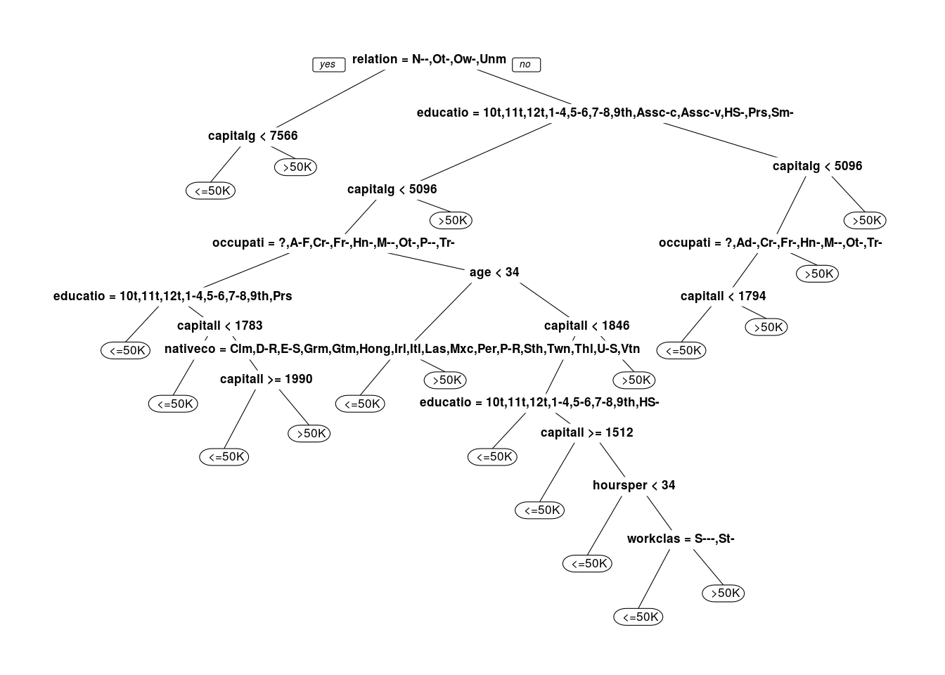

18

Conclusion

This highlights one important trade-off in building predictive models. By tuning cp, we improved our accuracy by over 1%, but our tree became significantly more complicated. In some applications, such an improvement in accuracy would be worth the loss in interpretability. In others, we may prefer a less accurate model that is simpler to understand and describe over a more accurate – but more complicated – model.

R Data Analytics Machine Learning

Rihad Variawa

Data Scientist

I am the Sr. Data Scientist at Malastare AI and head of global Fintech Research, responsible for overall vision and strategy, investment priorities and offering development. Working in the financial services industry, helping clients adopt new technologies that can transform the way they transact and engage with their customers. I am passionate about data science, super inquisitive and challenge seeker; looking at everything through a lens of numbers and problem-solver at the core. From understanding a business problem to collecting and visualizing data, until the stage of prototyping, fine-tuning and deploying models to real-world applications, I find the fulfillment of tackling challenges to solve complex problems using data.