Forecasting U.S. Federal Reserve Interest Rate Hikes

Apr 11, 2019

The federal funds rate is the key interest rate that the U.S. Federal Reserve uses to influence economic growth. The Federal Open Market Committee meets regularly to decide whether to increase, decrease, or maintain the target interest rate. Their choice has important ramifications that cascade through the economy, so the announcement of the interest rates is eagerly awaited each month.

In this analysis, I’ll use analytics to try to predict when the Fed will raise interest rates. I’ll look at monthly economic and political data dating back to the mid-1960’s. In this analysis, the dependent variable will be the binary outcome variable RaisedFedFunds, which takes value 1 if the federal funds rate was increased that month and 0 if it was lowered or stayed the same. For each month, the file federalFundsRate.csv.xz contains the following independent variables:

Date: The date the change was announced.
Chairman: The name of the Federal Reserve Chairman at the time the change was announced.
PreviousRate: The federal funds rate in the prior month.
Streak: The current streak of raising or not raising the rate, e.g. +8 indicates the rate has been increased 8 months in a row, whereas -3 indicates the rate has been lowered or stayed the same for 3 months in a row.
GDP: The U.S. Gross Domestic Product, in Billions of Chained 2009 US Dollars.
Unemployment: The unemployment rate in the U.S.
CPI: The Consumer Price Index, an indicator of inflation, in the U.S.
HomeownershipRate: The rate of homeownership in the U.S.
DebtAsPctGDP: The U.S. national debt as a percentage of GDP
DemocraticPres: Whether the sitting U.S. President is a Democrat (DemocraticPres=1) or a Republican (DemocraticPres=0)
MonthsUntilElection: The number of remaining months until the next U.S. presidential election.

Problem 1 - Loading the Data

Use the read.csv function to load the contents of federalFundsRate.csv.xz file into a dataframe called fedFunds, using stringsAsFactors=FALSE.

What proportion of months did the Fed raise the interest rate?

fedFunds <- read.csv("federalFundsRate.csv.xz")
str(fedFunds)

'data.frame':   585 obs. of  12 variables:
 $ Date               : Factor w/ 585 levels "1966-02-01","1966-03-01",..: 1 2 3 4 5 6 7 8 9 10 ...
 $ Chairman           : Factor w/ 8 levels "Bernanke, Ben",..: 4 4 4 4 4 4 4 4 4 4 ...
 $ PreviousRate       : num  4.42 4.6 4.65 4.67 4.9 5.17 5.3 5.53 5.4 5.53 ...
 $ Streak             : int  4 5 6 7 8 9 10 11 -1 1 ...
 $ GDP                : num  4202 4202 4202 4219 4219 ...
 $ Unemployment       : num  4 3.8 3.8 3.8 3.9 3.8 3.8 3.8 3.7 3.7 ...
 $ CPI                : num  31.9 32.1 32.2 32.3 32.4 ...
 $ HomeownershipRate  : num  63.5 63.5 63.5 63.2 63.2 63.2 63.3 63.3 63.3 63.8 ...
 $ DebtAsPctGDP       : num  40.3 4201.9 4201.9 39.2 4219.1 ...
 $ DemocraticPres     : int  1 1 1 1 1 1 1 1 1 1 ...
 $ MonthsUntilElection: int  33 32 31 30 29 28 27 26 25 24 ...
 $ RaisedFedFunds     : int  1 1 1 1 1 1 1 0 1 1 ...

summary(fedFunds)

         Date                   Chairman    PreviousRate   
 1966-02-01:  1   Greenspan, Alan   :221   Min.   : 0.070  
 1966-03-01:  1   Bernanke, Ben     : 96   1st Qu.: 3.290  
 1966-04-01:  1   Burns, Arthur     : 96   Median : 5.390  
 1966-05-01:  1   Volcker, Paul     : 96   Mean   : 5.651  
 1966-06-01:  1   Martin, William M.: 48   3rd Qu.: 7.880  
 1966-07-01:  1   Miller, G. William: 17   Max.   :19.100  
 (Other)   :579   (Other)           : 11                   
     Streak             GDP         Unemployment         CPI        
 Min.   :-16.000   Min.   : 4202   Min.   : 3.400   Min.   : 31.88  
 1st Qu.: -2.000   1st Qu.: 6039   1st Qu.: 5.000   1st Qu.: 63.40  
 Median :  1.000   Median : 8907   Median : 5.900   Median :129.10  
 Mean   :  1.094   Mean   : 9450   Mean   : 6.181   Mean   :127.71  
 3rd Qu.:  3.000   3rd Qu.:12956   3rd Qu.: 7.300   3rd Qu.:180.00  
 Max.   : 27.000   Max.   :16206   Max.   :10.800   Max.   :237.63  
                                                                    
 HomeownershipRate  DebtAsPctGDP      DemocraticPres   MonthsUntilElection
 Min.   :63.20     Min.   :   30.60   Min.   :0.0000   Min.   : 0.00      
 1st Qu.:64.20     1st Qu.:   62.35   1st Qu.:0.0000   1st Qu.:12.00      
 Median :64.80     Median : 6039.16   Median :0.0000   Median :24.00      
 Mean   :65.41     Mean   : 6317.32   Mean   :0.4256   Mean   :23.58      
 3rd Qu.:66.50     3rd Qu.:10529.38   3rd Qu.:1.0000   3rd Qu.:35.00      
 Max.   :69.20     Max.   :16205.59   Max.   :1.0000   Max.   :47.00      
                                                                          
 RaisedFedFunds  
 Min.   :0.0000  
 1st Qu.:0.0000  
 Median :1.0000  
 Mean   :0.5026  
 3rd Qu.:1.0000  
 Max.   :1.0000

table(fedFunds$RaisedFedFunds)


  0   1 
291 294

294 / (291 + 294)

[1] 0.5025641

Problem 2 - The Longest-Serving Fed Chair

Which Fed Reserve Chair has presided over the most interest rate decisions?

table(fedFunds$Chairman)


     Bernanke, Ben      Burns, Arthur    Greenspan, Alan 
                96                 96                221 
Martin, William M. Miller, G. William                N/A 
                48                 17                  2 
     Volcker, Paul      Yellen, Janet 
                96                  9

Greenspan, Alan

Problem 3 - Converting Variables to Factors

Convert the following variables to factors using the as.factor function:

Chairman
DemocraticPres
RaisedFedFunds

Which of the following methods requires the dependent variables be stored as a factor variable when training a model for classification?

str(fedFunds)

'data.frame':   585 obs. of  12 variables:
 $ Date               : Factor w/ 585 levels "1966-02-01","1966-03-01",..: 1 2 3 4 5 6 7 8 9 10 ...
 $ Chairman           : Factor w/ 8 levels "Bernanke, Ben",..: 4 4 4 4 4 4 4 4 4 4 ...
 $ PreviousRate       : num  4.42 4.6 4.65 4.67 4.9 5.17 5.3 5.53 5.4 5.53 ...
 $ Streak             : int  4 5 6 7 8 9 10 11 -1 1 ...
 $ GDP                : num  4202 4202 4202 4219 4219 ...
 $ Unemployment       : num  4 3.8 3.8 3.8 3.9 3.8 3.8 3.8 3.7 3.7 ...
 $ CPI                : num  31.9 32.1 32.2 32.3 32.4 ...
 $ HomeownershipRate  : num  63.5 63.5 63.5 63.2 63.2 63.2 63.3 63.3 63.3 63.8 ...
 $ DebtAsPctGDP       : num  40.3 4201.9 4201.9 39.2 4219.1 ...
 $ DemocraticPres     : int  1 1 1 1 1 1 1 1 1 1 ...
 $ MonthsUntilElection: int  33 32 31 30 29 28 27 26 25 24 ...
 $ RaisedFedFunds     : int  1 1 1 1 1 1 1 0 1 1 ...

fedFunds$Chairman <- as.factor(fedFunds$Chairman)
fedFunds$DemocraticPres <- as.factor(fedFunds$DemocraticPres)
fedFunds$RaisedFedFunds <- as.factor(fedFunds$RaisedFedFunds)
str(fedFunds)

'data.frame':   585 obs. of  12 variables:
 $ Date               : Factor w/ 585 levels "1966-02-01","1966-03-01",..: 1 2 3 4 5 6 7 8 9 10 ...
 $ Chairman           : Factor w/ 8 levels "Bernanke, Ben",..: 4 4 4 4 4 4 4 4 4 4 ...
 $ PreviousRate       : num  4.42 4.6 4.65 4.67 4.9 5.17 5.3 5.53 5.4 5.53 ...
 $ Streak             : int  4 5 6 7 8 9 10 11 -1 1 ...
 $ GDP                : num  4202 4202 4202 4219 4219 ...
 $ Unemployment       : num  4 3.8 3.8 3.8 3.9 3.8 3.8 3.8 3.7 3.7 ...
 $ CPI                : num  31.9 32.1 32.2 32.3 32.4 ...
 $ HomeownershipRate  : num  63.5 63.5 63.5 63.2 63.2 63.2 63.3 63.3 63.3 63.8 ...
 $ DebtAsPctGDP       : num  40.3 4201.9 4201.9 39.2 4219.1 ...
 $ DemocraticPres     : Factor w/ 2 levels "0","1": 2 2 2 2 2 2 2 2 2 2 ...
 $ MonthsUntilElection: int  33 32 31 30 29 28 27 26 25 24 ...
 $ RaisedFedFunds     : Factor w/ 2 levels "0","1": 2 2 2 2 2 2 2 1 2 2 ...

Random forest (randomForest)

Problem 4 - Splitting the dataframe into a Training & Testing Set

Obtain a random training/testing set split with:

set.seed(201)
library(caTools)
spl <- sample.split(fedFunds$RaisedFedFunds, 0.7)

Split months into a training dataframe called “training” using the observations for which spl is TRUE and a testing dataframe called “testing” using the observations for which spl is FALSE.

training <- subset(fedFunds, spl == TRUE)
testing <- subset(fedFunds, spl == FALSE)

Why do we use the sample.split() function to split into a training and testing set? #### It balances the dependent variable between the training and testing sets

Problem 5 - Training a Logistic Regression Model

Train a logistic regression model using independent variables “PreviousRate”, “Streak”, “Unemployment”, “HomeownershipRate”, “DemocraticPres”, and “MonthsUntilElection”, using the training set to obtain the model.

LogIntRate <- glm(RaisedFedFunds ~ PreviousRate + Streak + Unemployment +
                      HomeownershipRate + DemocraticPres + MonthsUntilElection, 
                  data = training, family = binomial)

Which of the following characteristics is the most statistically significant associated with an increased chance of the fed funds rate being raised?

summary(LogIntRate)


Call:
glm(formula = RaisedFedFunds ~ PreviousRate + Streak + Unemployment + 
    HomeownershipRate + DemocraticPres + MonthsUntilElection, 
    family = binomial, data = training)

Deviance Residuals: 
    Min       1Q   Median       3Q      Max  
-2.8177  -1.0121   0.2301   1.0491   2.5297  

Coefficients:
                     Estimate Std. Error z value Pr(>|z|)    
(Intercept)          9.121012   5.155774   1.769   0.0769 .  
PreviousRate        -0.003427   0.032350  -0.106   0.9156    
Streak               0.157658   0.025147   6.270 3.62e-10 ***
Unemployment        -0.047449   0.065438  -0.725   0.4684    
HomeownershipRate   -0.136451   0.076872  -1.775   0.0759 .  
DemocraticPres1      0.347829   0.233200   1.492   0.1358    
MonthsUntilElection -0.006931   0.007678  -0.903   0.3666    
---
Signif. codes:  0 '***' 0.001 '**' 0.01 '*' 0.05 '.' 0.1 ' ' 1

(Dispersion parameter for binomial family taken to be 1)

    Null deviance: 568.37  on 409  degrees of freedom
Residual deviance: 492.69  on 403  degrees of freedom
AIC: 506.69

Number of Fisher Scoring iterations: 4

A longer consecutive STREAK of months in which the fed funds rate was raised

Problem 6 - Predicting Using a Logistic Regression Model

Imagine you are an analyst at a bank and your manager has asked you to predict whether the fed funds rate will be raised next month.

You know that the rate has been lowered for 3 straight months (Streak = -3) and that the previous month’s rate was 1.7%.

The unemployment rate is 5.1% and the homeownership rate is 65.3%.

The current U.S. president is a Republican and the next election will be held in 18 months. According to the logistic regression model you built in Problem 5.

What is the predicted probability that the interest rate will be raised?

9.121012 + PreviousRate(-0.003427) + Streak0.157658 + Unemployment(-0.047449) + HomeownershipRate(-0.136451) + DemocraticPres10.347829 + MonthsUntilElection(-0.006931)

9.121012 + 1.7*(-0.003427) - 3*0.157658 + 
    5.1*(-0.047449) + 65.3*(-0.136451) + 
    0*0.347829 + 18*(-0.006931)

[1] -0.6347861

-0.6347861 ==> Need to plug it into the logistic response function

problem6 <- training[1, ]
problem6$PreviousRate <- 1.7
problem6$Streak <- -3
problem6$Unemployment <- 5.1
problem6$HomeownershipRate <- 65.3
problem6$DemocraticPres <- as.factor(0)
problem6$MonthsUntilElection <- 18
problem6

        Date           Chairman PreviousRate Streak      GDP Unemployment
1 1966-02-01 Martin, William M.          1.7     -3 4201.891          5.1
    CPI HomeownershipRate DebtAsPctGDP DemocraticPres MonthsUntilElection
1 31.88              65.3     40.26076              0                  18
  RaisedFedFunds
1              1

str(problem6)

'data.frame':   1 obs. of  12 variables:
 $ Date               : Factor w/ 585 levels "1966-02-01","1966-03-01",..: 1
 $ Chairman           : Factor w/ 8 levels "Bernanke, Ben",..: 4
 $ PreviousRate       : num 1.7
 $ Streak             : num -3
 $ GDP                : num 4202
 $ Unemployment       : num 5.1
 $ CPI                : num 31.9
 $ HomeownershipRate  : num 65.3
 $ DebtAsPctGDP       : num 40.3
 $ DemocraticPres     : Factor w/ 1 level "0": 1
 $ MonthsUntilElection: num 18
 $ RaisedFedFunds     : Factor w/ 2 levels "0","1": 2

problem6PredProb <- predict(LogIntRate, newdata = problem6, type = "response")
problem6PredProb

        1 
0.3464297

Problem 7 - Interpreting Model Coefficients

What is the meaning of the coefficient labeled “DemocraticPres1” in the logistic regression summary output?

summary(LogIntRate)


Call:
glm(formula = RaisedFedFunds ~ PreviousRate + Streak + Unemployment + 
    HomeownershipRate + DemocraticPres + MonthsUntilElection, 
    family = binomial, data = training)

Deviance Residuals: 
    Min       1Q   Median       3Q      Max  
-2.8177  -1.0121   0.2301   1.0491   2.5297  

Coefficients:
                     Estimate Std. Error z value Pr(>|z|)    
(Intercept)          9.121012   5.155774   1.769   0.0769 .  
PreviousRate        -0.003427   0.032350  -0.106   0.9156    
Streak               0.157658   0.025147   6.270 3.62e-10 ***
Unemployment        -0.047449   0.065438  -0.725   0.4684    
HomeownershipRate   -0.136451   0.076872  -1.775   0.0759 .  
DemocraticPres1      0.347829   0.233200   1.492   0.1358    
MonthsUntilElection -0.006931   0.007678  -0.903   0.3666    
---
Signif. codes:  0 '***' 0.001 '**' 0.01 '*' 0.05 '.' 0.1 ' ' 1

(Dispersion parameter for binomial family taken to be 1)

    Null deviance: 568.37  on 409  degrees of freedom
Residual deviance: 492.69  on 403  degrees of freedom
AIC: 506.69

Number of Fisher Scoring iterations: 4

When the president is Democratic, the odds of the fed funds rate increasing are 41.6% higher than in an otherise identical month (i.e. identical among the variables in the model). EXPLANATION:

The coefficients of the model are the log odds associated with that variable; so we see that the odds of being sold are exp(0.347829)=1.41599 those of an otherwise identical month. This means the month is predicted to have 41.6% higher odds of being sold.

Problem 8 - Obtaining Test Set Predictions

Using our logistic regression model, obtain predictions on the test-set. Then, using a probability threshold of 0.5, create a confusion matrix for the test-set.

On how many test-set observations does our logistic regression model make a different prediction than the prediction the naive baseline model would make?

(Remember that the naive baseline model we use always predicts the most frequent outcome in the training set for all observations in the test-set.)

str(testing)

'data.frame':   175 obs. of  12 variables:
 $ Date               : Factor w/ 585 levels "1966-02-01","1966-03-01",..: 14 15 16 18 19 31 32 37 38 39 ...
 $ Chairman           : Factor w/ 8 levels "Bernanke, Ben",..: 4 4 4 4 4 4 4 4 4 4 ...
 $ PreviousRate       : num  5 4.53 4.05 3.98 3.79 6.02 6.03 6.3 6.61 6.79 ...
 $ Streak             : int  1 -1 -2 1 -1 -2 1 2 3 4 ...
 $ GDP                : num  4325 4325 4329 4329 4366 ...
 $ Unemployment       : num  3.8 3.8 3.8 3.9 3.8 3.7 3.5 3.4 3.4 3.4 ...
 $ CPI                : num  33 33 33.1 33.3 33.4 34.9 35 35.7 35.8 36.1 ...
 $ HomeownershipRate  : num  63.3 63.3 63.9 63.9 63.8 64.1 64.1 64.1 64.1 64.1 ...
 $ DebtAsPctGDP       : num  4324.9 4324.9 37.9 4328.7 38.8 ...
 $ DemocraticPres     : Factor w/ 2 levels "0","1": 2 2 2 2 2 2 2 1 1 1 ...
 $ MonthsUntilElection: int  20 19 18 16 15 3 2 45 44 43 ...
 $ RaisedFedFunds     : Factor w/ 2 levels "0","1": 1 1 1 1 2 2 1 2 2 2 ...

PredProb <- predict(LogIntRate, newdata = testing, type = "response")
table(testing$RaisedFedFunds, PredProb >= 0.5)

   
    FALSE TRUE
  0    60   27
  1    31   57

table(training$RaisedFedFunds)


  0   1 
204 206

91 (60 + 31 were predicted less than 0.5)

Problem 9 - Computing Test-Set AUC

What is the test-set AUC of the logistic regression model?

library(ROCR)

Loading required package: gplots


Attaching package: 'gplots'

The following object is masked from 'package:stats':

    lowess

PredTestLogROCR <- prediction(PredProb, testing$RaisedFedFunds)
performance(PredTestLogROCR, "auc")@y.values

[[1]]
[1] 0.704023

Problem 10 - Interpreting AUC

What is the meaning of the AUC? #### The proportion of the time the model can differentiate between a randomly selected month during which the fed funds were raised and a randomly selected month during which the federal funds were not raised.

Problem 11 - ROC Curves

Which logistic regression threshold is associated with the upper-right corner of the ROC plot (true positive rate 1 and false positive rate 1)? #### 0

EXPLANATION

A model with threshold 0 predicts 1 for all observations, yielding a 100% true positive rate and a 100% false positive rate.

Problem 12 - ROC Curves

Plot the colorized ROC curve for the logistic regression model’s performance on the test-set. At roughly which logistic regression cut-off does the model achieve a true positive rate of 85% and a false positive rate of 60%?

ROCRperf <- performance(PredTestLogROCR, "tpr", "fpr")
plot(ROCRperf, colorize = TRUE, 
     print.cutoffs.at = seq(0, 1, by = 0.1), 
     text.adj = c(-0.2, 1.7))

0.37

Problem 13 - Cross-Validation to Select Parameters

Which of the following best describes how 10-fold cross-validation works when selecting between 2 different parameter values? #### 20 models are trained on subsets of the training set and evaluated on a portion of the training set

Problem 14 - Cross-Validation for a CART Model

Set the random seed to 201 (even though you have already done so earlier in the problem).

Then use the caret package and the train function to perform 10-fold cv with the training data set to select the best cp value for a CART model that predicts the dependent variable “RaisedFedFunds” using the independent variables “PreviousRate,” “Streak,” “Unemployment,” “HomeownershipRate,” “DemocraticPres,” and “MonthsUntilElection.” Select the cp value from a grid consisting of the 50 values 0.001, 0.002, …, 0.05.

library(caret)

Loading required package: lattice

Loading required package: ggplot2

library(e1071)
set.seed(201)

# define cross-validation experiment
numFolds <- trainControl(method = "cv", number = 10)
cpGrid <- expand.grid(.cp = seq(0.001, 0.05, 0.001))

Define cv experiment

numFolds <- trainControl(method = "cv", number = 10)
cpGrid <- expand.grid(.cp = seq(0.001, 0.05, 0.001))

Perform the cv

trainCV <- train(RaisedFedFunds ~ PreviousRate + Streak + Unemployment + 
                     HomeownershipRate + DemocraticPres + MonthsUntilElection, 
                 data = training, 
                 method = "rpart", 
                 trControl = numFolds, 
                 tuneGrid = cpGrid)
trainCV

CART 

410 samples
  6 predictor
  2 classes: '0', '1' 

No pre-processing
Resampling: Cross-Validated (10 fold) 
Summary of sample sizes: 369, 368, 368, 369, 370, 370, ... 
Resampling results across tuning parameters:

  cp     Accuracy   Kappa    
  0.001  0.6248461  0.2498288
  0.002  0.6366928  0.2737781
  0.003  0.6465099  0.2940348
  0.004  0.6465099  0.2940348
  0.005  0.6465099  0.2940348
  0.006  0.6513298  0.3037278
  0.007  0.6513298  0.3037278
  0.008  0.6488298  0.2987278
  0.009  0.6462108  0.2934897
  0.010  0.6437718  0.2887290
  0.011  0.6532956  0.3075752
  0.012  0.6532956  0.3075752
  0.013  0.6532956  0.3075752
  0.014  0.6386527  0.2782894
  0.015  0.6386527  0.2782894
  0.016  0.6386527  0.2782894
  0.017  0.6287718  0.2585275
  0.018  0.6287718  0.2585275
  0.019  0.6287718  0.2585275
  0.020  0.6385918  0.2780499
  0.021  0.6385918  0.2780499
  0.022  0.6385918  0.2784431
  0.023  0.6385918  0.2784431
  0.024  0.6432956  0.2882859
  0.025  0.6432956  0.2882859
  0.026  0.6605575  0.3228097
  0.027  0.6605575  0.3228097
  0.028  0.6680575  0.3378097
  0.029  0.6680575  0.3378097
  0.030  0.6680575  0.3381290
  0.031  0.6680575  0.3381290
  0.032  0.6680575  0.3381290
  0.033  0.6680575  0.3381290
  0.034  0.6680575  0.3381290
  0.035  0.6680575  0.3381290
  0.036  0.6729355  0.3474661
  0.037  0.6729355  0.3474661
  0.038  0.6729355  0.3474661
  0.039  0.6729355  0.3474661
  0.040  0.6729355  0.3474661
  0.041  0.6729355  0.3474661
  0.042  0.6729355  0.3474661
  0.043  0.6729355  0.3474661
  0.044  0.6729355  0.3474661
  0.045  0.6729355  0.3474661
  0.046  0.6729355  0.3474661
  0.047  0.6729355  0.3474661
  0.048  0.6729355  0.3474661
  0.049  0.6729355  0.3474661
  0.050  0.6729355  0.3474661

Accuracy was used to select the optimal model using the largest value.
The final value used for the model was cp = 0.05.

What cp value maximizes the cv accuracy? #### 0.016

Problem 15 - Train CART Model

Create and plot the CART model trained with the parameter identified in Problem 14, again predicting the dependent variable using “PreviousRate”, “Streak”, “Unemployment”, “HomeownershipRate”, “DemocraticPres”, and “MonthsUntilElection”.

What variable is used as the first (upper-most) split in the tree?

library(rpart)
library(rpart.plot)
TreeIntRate <- trainCV$finalModel
prp(TreeIntRate)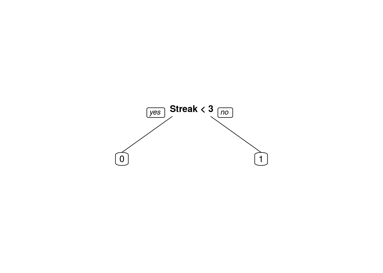

TreeIntRate

n= 410 

node), split, n, loss, yval, (yprob)
      * denotes terminal node

1) root 410 204 1 (0.4975610 0.5024390)  
  2) Streak< 2.5 300 115 0 (0.6166667 0.3833333) *
  3) Streak>=2.5 110  19 1 (0.1727273 0.8272727) *

TreeIntRate2 <- rpart(RaisedFedFunds ~ PreviousRate + Streak + Unemployment + 
                          HomeownershipRate + DemocraticPres + 
                          MonthsUntilElection, 
                      data = training, 
                      method = "class", 
                      cp = 0.016)
prp(TreeIntRate2)

Streak

Problem 16 - Predicting Using a CART Model

If you were to use the CART model you created in Problem 15 to explore the question asked of the analyst in Problem 6, what would you predict for next month?

Remember: The rate has been lowered for 3 straight months (Streak = -3). The previous month’s rate was 1.7%. The unemployment rate is 5.1%. The homeownership rate is 65.3%. The current U.S. president is a Republican and the next election will be held in 18 months. #### The Fed will not raise the federal funds rate. The Fed will not raise the fed funds rate.

Problem 17 - Test-Set Accuracy for CART Model

Using the CART model you created in Problem 15, obtain predictions on the test-set (using the parameter type=“class” with the predict function).

Then, create a confusion matrix for the test-set.

PredClassTree <- predict(TreeIntRate2, newdata = testing, type = "class")

What is the accuracy of your CART model?

table(PredClassTree, testing$RaisedFedFunds)

             
PredClassTree  0  1
            0 64 40
            1 23 48

(64 + 48) / nrow(testing)

[1] 0.64

R Data Analytics Machine Learning

Rihad Variawa

Data Scientist

I am the Sr. Data Scientist at Malastare AI and head of global Fintech Research, responsible for overall vision and strategy, investment priorities and offering development. Working in the financial services industry, helping clients adopt new technologies that can transform the way they transact and engage with their customers. I am passionate about data science, super inquisitive and challenge seeker; looking at everything through a lens of numbers and problem-solver at the core. From understanding a business problem to collecting and visualizing data, until the stage of prototyping, fine-tuning and deploying models to real-world applications, I find the fulfillment of tackling challenges to solve complex problems using data.