
Flu epidemics constitute a major public health concern causing respiratory illnesses, hospitalizations, and deaths. According to the National Vital Statistics Reports published in October 2012, influenza ranked as the eighth leading cause of death in 2011 in the U.S. Each year, 250,000 to 500,000 deaths are attributed to influenza related diseases throughout the world.
The U.S. Centers for Disease Control and Prevention (CDC) and the European Influenza Surveillance Scheme (EISS) detect influenza activity through virologic and clinical data, including Influenza-like Illness (ILI) physician visits. Reporting national and regional data, however, are published with a 1-2 week lag.
The Google Flu Trends project was initiated to see if faster reporting can be made possible by considering flu-related online search queries – data that is available almost immediately.
I would like to estimate influenza-like illness (ILI) activity using Google web search logs. Fortunately, one can easily access this data online:
- ILI Data - The CDC publishes on its website the official regional and state-level percentage of patient visits to healthcare providers for ILI purposes on a weekly basis.
- Google Search Queries - Google Trends allows public retrieval of weekly counts for every query searched by users around the world.
For each location, the counts are normalized by dividing the count for each query in a particular week by the total number of online search queries submitted in that location during the week. Then, the values are adjusted to be between 0 and 1.
The csv file FluTrain.csv aggregates this data from January 1, 2004 until December 31, 2011 as follows:
- “Week” - The range of dates represented by this observation, in year/month/day format.
- “ILI” - This column lists the percentage of ILI-related physician visits for the corresponding week.
- “Queries” - This column lists the fraction of queries that are ILI-related for the corresponding week, adjusted to be between 0 and 1 (higher values correspond to more ILI-related search queries).
Before applying analytics tools on the training set, we first need to understand the data at hand. Looking at the time period 2004-2011, which week corresponds to the highest percentage of ILI-related physician visits?
Loading the data
FluTrain <- read.csv("FluTrain.csv")
summary(FluTrain)
Week ILI Queries
2004-01-04 - 2004-01-10: 1 Min. :0.5341 Min. :0.04117
2004-01-11 - 2004-01-17: 1 1st Qu.:0.9025 1st Qu.:0.15671
2004-01-18 - 2004-01-24: 1 Median :1.2526 Median :0.28154
2004-01-25 - 2004-01-31: 1 Mean :1.6769 Mean :0.28603
2004-02-01 - 2004-02-07: 1 3rd Qu.:2.0587 3rd Qu.:0.37849
2004-02-08 - 2004-02-14: 1 Max. :7.6189 Max. :1.00000
(Other) :411 str(FluTrain)'data.frame': 417 obs. of 3 variables:
$ Week : Factor w/ 417 levels "2004-01-04 - 2004-01-10",..: 1 2 3 4 5 6 7 8 9 10 ...
$ ILI : num 2.42 1.81 1.71 1.54 1.44 ...
$ Queries: num 0.238 0.22 0.226 0.238 0.224 ...Problem 1.1 - EDA
Select the day of the month corresponding to the start of this week?
FluTrain[which.max(FluTrain$ILI),] Week ILI Queries
303 2009-10-18 - 2009-10-24 7.618892 1Which week corresponds to the highest percentage of ILI-related query fraction?
FluTrain[which.max(FluTrain$Queries),] Week ILI Queries
303 2009-10-18 - 2009-10-24 7.618892 1subset(FluTrain, Queries == 1) Week ILI Queries
303 2009-10-18 - 2009-10-24 7.618892 1October 18, 2009
Problem 1.2 - EDA
Let’s now understand the data at a high level. Plot the histogram of the dependent variable, ILI.
What best describes the distribution of values of ILI?
hist(FluTrain$ILI)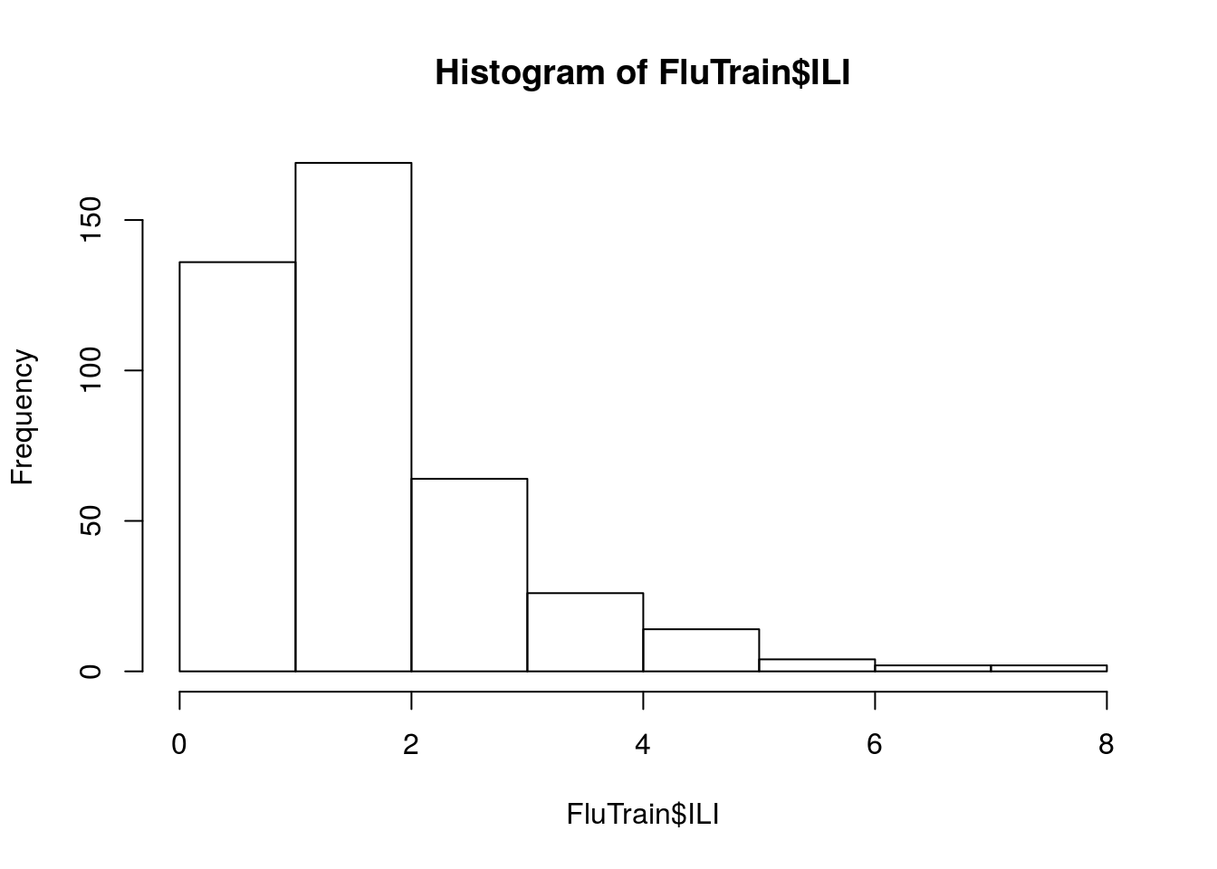
Most of the ILI values are small, with a relatively small number of much larger values (in statistics, this sort of data is called “skew right”).
Problem 1.3 - EDA
When handling a skewed dependent variable, it is often useful to predict the logarithm of the dependent variable instead of the dependent variable itself – this prevents the small number of unusually large or small observations from having an undue influence on the sum of squared errors of predictive models.
In this problem, I’ll predict the natural log of the ILI variable, which can be computed using the log() function. Plot the natural logarithm of ILI versus Queries.
plot(log(FluTrain$ILI), FluTrain$Queries)
plot(FluTrain$Queries, log(FluTrain$ILI))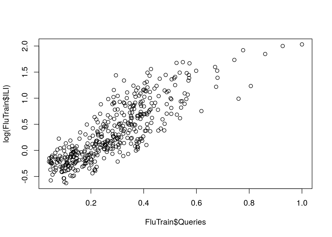
What does the plot suggest? #### There is a positive, linear relationship between log(ILI) and Queries.
Problem 2.1 - Linear Regression Model
Based on the plot we just made, it seems that a linear regression model could be a good modeling choice. Based on our understanding of the data from the previous subproblem, which model best describes our estimation problem? #### log(ILI) = intercept + coefficient x Queries, where the coefficient is positive.
Problem 2.2 - Linear Regression Model
Let’s call the regression model from the previous problem (Problem 2.1). FluTrend1 and run it. Hint: to take the logarithm of a variable Var in a regression equation, you simply use log(Var) when specifying the formula to the lm() function.
FluTrend1 <- lm(log(ILI) ~ Queries, data = FluTrain)What is the training set R-squared value for FluTrend1 model (the “Multiple R-squared”)?
summary(FluTrend1)
Call:
lm(formula = log(ILI) ~ Queries, data = FluTrain)

Residuals:
     Min       1Q   Median       3Q      Max
-0.76003 -0.19696 -0.01657  0.18685  1.06450

Coefficients:
            Estimate Std. Error t value Pr(>|t|)
(Intercept) -0.49934    0.03041  -16.42   <2e-16 ***
Queries      2.96129    0.09312   31.80   <2e-16 ***
---
Signif. codes:  0 '***' 0.001 '**' 0.01 '*' 0.05 '.' 0.1 ' ' 1

Residual standard error: 0.2995 on 415 degrees of freedom
Multiple R-squared:  0.709, Adjusted R-squared:  0.7083
F-statistic:  1011 on 1 and 415 DF,  p-value: < 2.2e-16
0.709
Problem 2.3 - Linear Regression Model
For a single variable linear regression model, there is a direct relationship between the R-squared and the correlation between the independent and the dependent variables.
What is the relationship we infer from our problem? (Don’t forget that you can use the cor function to compute the correlation between two variables.)
corILIQueries <- cor(log(FluTrain$ILI), FluTrain$Queries)
cor(FluTrain$ILI, FluTrain$Queries)
[1] 0.8142115corILIQueries^2[1] 0.7090201log(1/corILIQueries)[1] 0.1719357exp(-0.5 * corILIQueries)[1] 0.6563792Note = R-squared = Correlation^2
Note that the “exp” function stands for the exponential function. The exponential can be computed in R using the function exp().
Problem 3.1 - Performance on the Test Set
The file provides the 2012 weekly data of the ILI-related search queries and the observed weekly percentage of ILI-related physician visits.
Load this data into a dataframe called FluTest.
FluTest <- read.csv("FluTest.csv")Normally, we would obtain test-set predictions from the model FluTrend1 using the code PredTest1 = predict(FluTrend1, newdata=FluTest) However, the dependent variable in our model is log(ILI), so PredTest1 would contain predictions of the log(ILI) value.
We are instead interested in obtaining predictions of the ILI value. We can convert from predictions of log(ILI) to predictions of ILI via exponentiation, or the exp() function. The new code, which predicts the ILI value.
PredTest1 = exp(predict(FluTrend1, newdata=FluTest))What is our estimate for the percentage of ILI-related physician visits for the week of March 11, 2012? (HINT: You can either just output FluTest$Week to find which element corresponds to March 11, 2012, or you can use the “which” function in R. To learn more about the which function, type ?which in your R console.)
FluTest$Week [1] 2012-01-01 - 2012-01-07 2012-01-08 - 2012-01-14
[3] 2012-01-15 - 2012-01-21 2012-01-22 - 2012-01-28
[5] 2012-01-29 - 2012-02-04 2012-02-05 - 2012-02-11
[7] 2012-02-12 - 2012-02-18 2012-02-19 - 2012-02-25
[9] 2012-02-26 - 2012-03-03 2012-03-04 - 2012-03-10
[11] 2012-03-11 - 2012-03-17 2012-03-18 - 2012-03-24
[13] 2012-03-25 - 2012-03-31 2012-04-01 - 2012-04-07
[15] 2012-04-08 - 2012-04-14 2012-04-15 - 2012-04-21
[17] 2012-04-22 - 2012-04-28 2012-04-29 - 2012-05-05
[19] 2012-05-06 - 2012-05-12 2012-05-13 - 2012-05-19
[21] 2012-05-20 - 2012-05-26 2012-05-27 - 2012-06-02
[23] 2012-06-03 - 2012-06-09 2012-06-10 - 2012-06-16
[25] 2012-06-17 - 2012-06-23 2012-06-24 - 2012-06-30
[27] 2012-07-01 - 2012-07-07 2012-07-08 - 2012-07-14
[29] 2012-07-15 - 2012-07-21 2012-07-22 - 2012-07-28
[31] 2012-07-29 - 2012-08-04 2012-08-05 - 2012-08-11
[33] 2012-08-12 - 2012-08-18 2012-08-19 - 2012-08-25
[35] 2012-08-26 - 2012-09-01 2012-09-02 - 2012-09-08
[37] 2012-09-09 - 2012-09-15 2012-09-16 - 2012-09-22
[39] 2012-09-23 - 2012-09-29 2012-09-30 - 2012-10-06
[41] 2012-10-07 - 2012-10-13 2012-10-14 - 2012-10-20
[43] 2012-10-21 - 2012-10-27 2012-10-28 - 2012-11-03
[45] 2012-11-04 - 2012-11-10 2012-11-11 - 2012-11-17
[47] 2012-11-18 - 2012-11-24 2012-11-25 - 2012-12-01
[49] 2012-12-02 - 2012-12-08 2012-12-09 - 2012-12-15
[51] 2012-12-16 - 2012-12-22 2012-12-23 - 2012-12-29
52 Levels: 2012-01-01 - 2012-01-07 ... 2012-12-23 - 2012-12-29FluTest[11, ] Week ILI Queries
11 2012-03-11 - 2012-03-17 2.293422 0.4329349PredTest1[11] 11
2.187378 2.293422
Problem 3.2 - Performance on the Test Set
What is the relative error betweeen the estimate (our prediction) and the observed value for the week of March 11, 2012? Note that the relative error is calculated as (Observed ILI - Estimated ILI)/Observed ILI.
(FluTest[11, 2] - PredTest1[11]) / FluTest[11, 2] 11
0.04623827 Problem 3.3 - Performance on the Test Set
What is the Root Mean Square Error (RMSE) between our estimates and the actual observations for the percentage of ILI-related physician visits, on the test-set?
FluTestSSE = sum((PredTest1 - FluTest$ILI)^2)
FluTestRMSE = sqrt(FluTestSSE/nrow(FluTest))
FluTestRMSE
[1] 0.7490645Problem 4.1 - Training a Time Series Model
The observations in this dataset are consecutive weekly measurements of the dependent and independent variables. This sort of dataset is called a “time series.”
Often, statistical models can be improved by predicting the current value of the dependent variable using the value of the dependent variable from earlier weeks. In our models, this means we will predict the ILI variable in the current week using values of the ILI variable from previous weeks.
First, we need to decide the amount of time to lag the observations. Because the ILI variable is reported with a 1- or 2-week lag, a decision maker cannot rely on the previous week’s ILI value to predict the current week’s value. Instead, the decision maker will only have data available from 2 or more weeks ago.
We will build a variable called ILILag2 that contains the ILI value from 2 weeks before the current observation.
To do so, we’ll use the “zoo” package, which provides a number of helpful methods for time series models. While many functions are built into R, you need to add new packages to use some functions. New packages can be installed and loaded easily in R. Run the following two codes to install and load the zoo package.
In the first code, you will be prompted to select a CRAN mirror to use for your download. Select a mirror near you geographically. install.packages(“zoo”)
After installing and loading the zoo package, create the ILILag2 variable in the training set.
ILILag2 = lag(zoo(FluTrain$ILI), -2, na.pad=TRUE)
FluTrain$ILILag2 = coredata(ILILag2)
The value of -2 passed to lag means to return 2 observations before the current one; a positive value would have returned future observations. The parameter na.pad=TRUE means to add missing values for the first two weeks of our dataset, where we can’t compute the data from 2 weeks earlier.
?lag
?coredata
ILILag2
1 2 3 4 5 6 7
NA NA 2.4183312 1.8090560 1.7120239 1.5424951 1.4378683
8 9 10 11 12 13 14
1.3242740 1.3072567 1.0369770 1.0103204 1.0524925 1.0200901 0.9244187
15 16 17 18 19 20 21
0.7906450 0.8026098 0.8361300 0.7924358 0.6835877 0.7574523 0.7885854
22 23 24 25 26 27 28
0.8121710 0.8044629 0.8777009 0.7414530 0.6610222 0.7151092 0.5622412
29 30 31 32 33 34 35
0.7868082 0.8606578 0.6899440 0.7796912 0.6281439 0.9024586 0.8064432
36 37 38 39 40 41 42
0.8748878 0.9932130 0.8761408 0.9480916 0.9269426 0.9716430 0.8971591
43 44 45 46 47 48 49
1.0224828 1.0629632 1.1469570 1.2049501 1.3051655 1.2869916 1.5946756
50 51 52 53 54 55 56
1.3971432 1.4499567 1.6174545 2.1911192 2.5664893 2.1764491 2.2017121
57 58 59 60 61 62 63
2.5301211 3.0652381 3.9806083 4.5956803 4.7519706 4.1796206 3.4535851
64 65 66 67 68 69 70
3.1585224 2.6732010 2.3516104 1.8924285 1.5249048 1.4113441 1.2506826
71 72 73 74 75 76 77
1.2070250 1.0789550 1.1452080 1.0612426 1.0567977 1.2519310 1.0141893
78 79 80 81 82 83 84
1.0419693 0.9540274 0.8482299 0.8418715 0.7308936 0.7134316 0.6706772
85 86 87 88 89 90 91
0.6892776 0.7049290 0.6159033 0.6094256 0.6802587 0.7754884 0.6834214
92 93 94 95 96 97 98
0.7810748 0.8069435 1.0763468 1.0586890 1.1152326 1.1238125 1.2548892
99 100 101 102 103 104 105
1.3366090 1.3786364 1.6082900 1.4831056 1.6537399 2.0067892 2.5685716
106 107 108 109 110 111 112
3.0527762 2.4250373 2.0019506 2.0586902 2.2127697 2.3222001 2.4927920
113 114 115 116 117 118 119
2.7948942 2.9691114 2.8395905 2.7779902 2.4728693 2.1806146 2.0167951
120 121 122 123 124 125 126
1.6410133 1.3582865 1.1427983 1.0403125 0.9643469 0.9379817 0.9474493
127 128 129 130 131 132 133
0.8919182 0.8646427 0.9703199 0.8443901 0.7748704 0.8213725 0.8727445
134 135 136 137 138 139 140
0.9226345 0.8994868 0.8430824 0.8818244 0.8171452 0.8715001 0.7386205
141 142 143 144 145 146 147
0.7979660 1.0139373 0.8809358 0.9433663 0.8915462 1.2032228 1.0578822
148 149 150 151 152 153 154
1.1305354 1.1255230 1.2080820 1.3495244 1.4689004 1.8276716 1.6656012
155 156 157 158 159 160 161
1.8596834 2.3889130 2.7897759 3.1154858 2.2694245 1.8635464 1.9998635
162 163 164 165 166 167 168
2.4406044 2.8301821 3.1234256 3.2701949 3.1775688 2.7236366 2.5020140
169 170 171 172 173 174 175
2.4271992 1.9604132 1.5913980 1.3697835 1.3631668 1.1736951 1.0635756
176 177 178 179 180 181 182
0.9697111 0.9653617 0.8567489 0.8633465 0.9353695 0.7455694 0.7404281
183 184 185 186 187 188 189
0.6728965 0.6662820 0.6627473 0.5456190 0.5862306 0.6606867 0.5340928
190 191 192 193 194 195 196
0.5855491 0.6180750 0.6874647 0.7156961 0.8293131 0.8009115 0.9184839
197 198 199 200 201 202 203
0.8142590 1.0719708 1.2178574 1.2457554 1.3598449 1.4467085 1.5328638
204 205 206 207 208 209 210
1.6665324 1.9748773 1.6730547 1.6340509 1.7459475 1.9364319 2.4890534
211 212 213 214 215 216 217
2.2540484 2.0914715 2.3593428 3.3233143 4.4338100 5.3454714 5.4225751
218 219 220 221 222 223 224
5.3030330 4.2445550 3.6280001 3.0346275 2.5359536 2.0573015 1.7415035
225 226 227 228 229 230 231
1.4065217 1.2686070 1.0771887 0.9934452 0.9112119 0.9721091 0.9932575
232 233 234 235 236 237 238
1.0913202 0.8884460 0.8876915 0.8831874 0.8267564 0.7832014 0.7806103
239 240 241 242 243 244 245
0.7690726 0.7212979 0.7525273 0.7527210 0.7927660 0.7438962 0.8141663
246 247 248 249 250 251 252
0.8384009 0.8511236 1.1097575 1.0311436 1.0228436 1.0301739 1.0124478
253 254 255 256 257 258 259
1.0835911 1.1657765 1.1912964 1.2807470 1.2705251 1.5957825 1.4584994
260 261 262 263 264 265 266
1.4992072 1.6298157 2.1556121 2.0205270 1.5456623 1.6422367 1.9652378
267 268 269 270 271 272 273
2.3436784 2.8605744 3.3421049 3.2056588 3.1004908 2.9581850 2.4638058
274 275 276 277 278 279 280
2.1927224 1.8739459 1.6481690 1.4987776 1.2923267 1.2716411 2.9815890
281 282 283 284 285 286 287
2.4370224 2.2813011 3.8157199 4.2131523 3.1783224 2.5097162 2.0663177
288 289 290 291 292 293 294
1.7180460 1.5596467 1.3085629 1.1869460 1.1379623 1.1500523 1.1126189
295 296 297 298 299 300 301
1.1614188 1.6410714 2.4716598 3.7196936 3.9497480 4.0875636 4.0189724
302 303 304 305 306 307 308
4.6036164 5.6608671 6.8152222 7.6188921 7.3883586 6.3392723 4.9434950
309 310 311 312 313 314 315
3.8099612 3.4410588 2.6677306 2.4718250 2.3449995 2.7143498 2.6766718
316 317 318 319 320 321 322
1.9828382 1.8274862 1.9260563 1.9249472 2.0887684 2.0343408 1.9764946
323 324 325 326 327 328 329
1.9936177 1.8538260 1.8673036 1.6998677 1.4974082 1.4511188 1.2071478
330 331 332 333 334 335 336
1.1741508 1.1620668 1.1721343 1.1216765 1.1498116 1.1332758 1.0817133
337 338 339 340 341 342 343
1.1995860 0.9528083 0.9160321 0.9265822 0.8696197 0.9031331 0.7737757
344 345 346 347 348 349 350
0.7427744 0.7309345 0.7868818 0.7630507 0.8410432 0.7915728 0.9127318
351 352 353 354 355 356 357
1.0339765 0.9340091 1.0818888 1.0656260 1.1350529 1.2525629 1.2456956
358 359 360 361 362 363 364
1.2677380 1.4372295 1.5334125 1.6944544 1.9915024 1.8130453 2.0142579
365 366 367 368 369 370 371
2.5565913 3.3818486 3.4317231 2.6915111 2.9106289 3.4923189 4.0036963
372 373 374 375 376 377 378
4.4353368 4.2421482 4.3971861 3.9025565 3.1507275 2.7242234 2.3333563
379 380 381 382 383 384 385
1.9250003 1.7524260 1.5770365 1.3576558 1.3122310 1.1493747 1.1145057
386 387 388 389 390 391 392
1.1098449 1.0524026 1.0353647 1.1177658 0.9829495 0.9251944 0.8355311
393 394 395 396 397 398 399
0.8323927 0.8555910 0.7069494 0.6943868 0.6879762 0.6447430 0.6753299
400 401 402 403 404 405 406
0.7282297 0.8065263 0.8604084 0.9360754 0.9666827 0.9960071 1.1084635
407 408 409 410 411 412 413
1.2030858 1.2369566 1.2525865 1.3054612 1.4528432 1.4408922 1.4622115
414 415 416 417
1.6554147 1.4657230 1.5181061 1.6639544 How many values are missing in the new ILILag2 variable?
sum(is.na(FluTrain$ILILag2))[1] 2Problem 4.2 - Training a Time Series Model
Use the plot() function to plot the log of ILILag2 against the log of ILI.
Which best describes the relationship between these two variables?
plot(log(FluTrain$ILILag2), log(FluTrain$ILI))
There is a strong positive relationship between log(ILILag2) and log(ILI).
Problem 4.3 - Training a Time Series Model
Train a linear regression model on the FluTrain dataset to predict the log of the ILI variable using the Queries variable as well as the log of the ILILag2 variable. Call this model FluTrend2.
FluTrend2 <- lm(log(ILI) ~ Queries + log(ILILag2), data = FluTrain)Which coefficients are significant at the p=0.05 level in this regression model?
summary(FluTrend2)
Call:
lm(formula = log(ILI) ~ Queries + log(ILILag2), data = FluTrain)

Residuals:
     Min       1Q   Median       3Q      Max
-0.52209 -0.11082 -0.01819  0.08143  0.76785

Coefficients:
             Estimate Std. Error t value Pr(>|t|)
(Intercept)  -0.24064    0.01953  -12.32   <2e-16 ***
Queries       1.25578    0.07910   15.88   <2e-16 ***
log(ILILag2)  0.65569    0.02251   29.14   <2e-16 ***
---
Signif. codes:  0 '***' 0.001 '**' 0.01 '*' 0.05 '.' 0.1 ' ' 1

Residual standard error: 0.1703 on 412 degrees of freedom
  (2 observations deleted due to missingness)
Multiple R-squared:  0.9063,    Adjusted R-squared:  0.9059
F-statistic:  1993 on 2 and 412 DF,  p-value: < 2.2e-16
All are significant at p<0.05
What is the R^2 value of the FluTrend2 model? #### 0.9063
Problem 4.4 - Training a Time Series Model
On the basis of R-squared value and significance of coefficients, which statement is the most accurate?
summary(FluTrend1)
Call:
lm(formula = log(ILI) ~ Queries, data = FluTrain)

Residuals:
     Min       1Q   Median       3Q      Max
-0.76003 -0.19696 -0.01657  0.18685  1.06450

Coefficients:
            Estimate Std. Error t value Pr(>|t|)
(Intercept) -0.49934    0.03041  -16.42   <2e-16 ***
Queries      2.96129    0.09312   31.80   <2e-16 ***
---
Signif. codes:  0 '***' 0.001 '**' 0.01 '*' 0.05 '.' 0.1 ' ' 1

Residual standard error: 0.2995 on 415 degrees of freedom
Multiple R-squared:  0.709, Adjusted R-squared:  0.7083
F-statistic:  1011 on 1 and 415 DF,  p-value: < 2.2e-16
summary(FluTrend2)
Call:
lm(formula = log(ILI) ~ Queries + log(ILILag2), data = FluTrain)

Residuals:
     Min       1Q   Median       3Q      Max
-0.52209 -0.11082 -0.01819  0.08143  0.76785

Coefficients:
             Estimate Std. Error t value Pr(>|t|)
(Intercept)  -0.24064    0.01953  -12.32   <2e-16 ***
Queries       1.25578    0.07910   15.88   <2e-16 ***
log(ILILag2)  0.65569    0.02251   29.14   <2e-16 ***
---
Signif. codes:  0 '***' 0.001 '**' 0.01 '*' 0.05 '.' 0.1 ' ' 1

Residual standard error: 0.1703 on 412 degrees of freedom
  (2 observations deleted due to missingness)
Multiple R-squared:  0.9063,    Adjusted R-squared:  0.9059
F-statistic:  1993 on 2 and 412 DF,  p-value: < 2.2e-16
FluTrend2 is a stronger model than FluTrend1 on the training set, due to it’s higher R^2 value.
Problem 5.1 - Evaluating the Time Series Model in the Test Set
So far, we have only added the ILILag2 variable to the FluTrain dataframe. To make predictions with our FluTrend2 model, we’ll also need to add ILILag2 to the FluTest dataframe (note that adding variables before splitting into a training and testing set can prevent this duplication of effort).
Modifying the code from the previous subproblem to add an ILILag2 variable to the FluTest dataframe.
How many missing values are there in this new variable?
Test_ILILag2 = lag(zoo(FluTest$ILI), -2, na.pad=TRUE)
FluTest$ILILag2 = coredata(Test_ILILag2)
sum(is.na(FluTest$ILILag2))
[1] 2Problem 5.2 - Evaluating the Time Series Model in the Test Set
In this problem, the training and testing sets are split sequentially – the training set contains all observations from 2004-2011 and the testing set contains all observations from 2012.
There is no time gap between the two datasets, meaning the first observation in FluTest was recorded one week after the last observation in FluTrain. From this, we can identify how to fill in the missing values for the ILILag2 variable in FluTest. Which value should be used to fill in the ILILag2 variable for the first observation in FluTest?
The ILI value of the second-to-last observation in the FluTrain dataframe. Which value should be used to fill in the ILILag2 variable for the second observation in FluTest? #### The ILI value of the last observation in the FluTrain dataframe.
Problem 5.3 - Evaluating the Time Series Model in the Test Set
Fill in the missing values for ILILag2 in FluTest. In terms of syntax, you could set the value of ILILag2 in row “x” of the FluTest dataframe to the value of ILI in row “y” of the FluTrain dataframe with “FluTest\(ILILag2[x] = FluTrain\)ILI[y]”.
Use the answer to the previous questions to determine the appropriate values of “x” and “y”. It may be helpful to check the total number of rows in FluTrain using str(FluTrain) or nrow(FluTrain).
nrow(FluTrain)[1] 417FluTest$ILILag2[1] = FluTrain$ILI[416]
FluTest$ILILag2[2] = FluTrain$ILI[417]What is the new value of the ILILag2 variable in the first row of FluTest?
FluTrain$ILI[416][1] 1.852736FluTest$ILILag2[1][1] 1.852736What is the new value of the ILILag2 variable in the second row of FluTest?
FluTrain$ILI[417][1] 2.12413FluTest$ILILag2[2][1] 2.12413Problem 5.4 - Evaluating the Time Series Model in the Test Set
Obtain test-set predictions of the ILI variable from the FluTrend2 model, again remembering to call the exp() function on the result of the predict() function to obtain predictions for ILI instead of log(ILI).
What is the test-set RMSE of the FluTrend2 model?
PredTest2 = exp(predict(FluTrend2, newdata=FluTest))
FluTestSSE2 = sum((PredTest2 - FluTest$ILI)^2)
FluTestRMSE2 = sqrt(FluTestSSE2/nrow(FluTest))
FluTestRMSE2
[1] 0.2942029Problem 5.5 - Evaluating the Time Series Model in the Test Set
Which model obtained the best test-set RMSE? #### FluTrend2 (less RMSE is better)
Conclusion
In this analysis, I’ve used a simple time series model with a single lag term. ARIMA models are a more general form of the model we built, which can include multiple lag terms as well as more complicated combinations of previous values of the dependent variable.
)